CS285 DRL Notes-Lecture 6 Actor-Critic

This is the note for Berkeley CS285 Lecture 6. The lecture turns REINFORCE into actor-critic by learning a value function that gives each action a less noisy credit signal.

The actor decides what to do; the critic estimates how much that decision improves the future. Actor-critic is therefore policy gradient with learned credit assignment.

Why add a critic?

REINFORCE weights an action by one sampled reward-to-go. That sample is correct on average, but it contains randomness from every later transition and action.

Lecture 6 keeps the value-function notation from Lecture 4 and defines

$$ \begin{aligned} Q^\pi(s_t,a_t) &=\sum_{t'=t}^{H} \mathbb E_{\pi_\theta} [r(s_{t'},a_{t'})\mid s_t,a_t],\\ V^\pi(s_t) &=\mathbb{E}_{a_t\sim\pi_\theta(a_t\mid s_t)} [Q^\pi(s_t,a_t)],\\ A^\pi(s_t,a_t) &=Q^\pi(s_t,a_t)-V^\pi(s_t). \end{aligned} $$

$Q^\pi$ asks how good one action is, $V^\pi$ asks how good the state is under the policy, and $A^\pi$ asks whether the action is better or worse than the policy’s usual action at that state.

The policy-gradient estimator becomes

$$ \nabla_\theta J(\theta) \approx \frac{1}{N}\sum_{i=1}^{N}\sum_{t=1}^{H} \nabla_\theta\log\pi_\theta(a_t^{(i)}\mid s_t^{(i)}) A^\pi(s_t^{(i)},a_t^{(i)}). $$

The actor is still updated through $\log\pi_\theta$. This formula uses the exact $A^\pi$; the practical question is how to construct a useful estimate $\hat A^\pi(s_t,a_t)$ from samples.

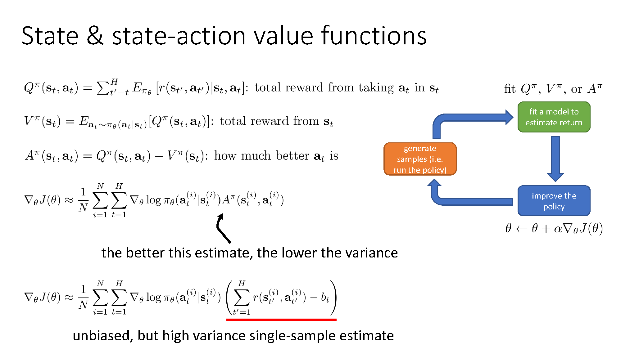
The critic does not predict the action and does not replace the reward. It averages over possible futures so that the actor does not have to learn from raw trajectory noise.

How can the critic learn a value with no labels?

For a fixed policy $\pi$, estimating its value is called policy evaluation. The policy-evaluation slides now introduce a discount $\gamma$; setting $\gamma=1$ recovers the finite-horizon definitions above. The Bellman identity supplies the structure:

$$ V^\pi(s_t) =\mathbb{E}_{a_t\sim\pi_\theta(a_t\mid s_t)} \left[ r(s_t,a_t)+\gamma \mathbb{E}_{s_{t+1}\sim p(s_{t+1}\mid s_t,a_t)} [V^\pi(s_{t+1})] \right]. $$

This is an identity for the true value function, not yet a training rule. We can turn it into two kinds of regression targets.

Monte Carlo target

Wait until the trajectory ends and use the observed return

$$ G_t=\sum_{t'=t}^{H}\gamma^{t'-t}r(s_{t'},a_{t'}). $$

Then fit the lecture’s value estimator $\hat V_\phi^\pi$ by minimizing

$$ \mathcal L(\phi) =\frac{1}{2}\sum_{i=1}^{N}\sum_{t=1}^{H} \left\|\hat V_\phi^\pi(s_t^{(i)})-G_t^{(i)}\right\|^2. $$

$G_t$ uses the real future, so it does not inherit approximation error from the critic. Its weakness is variance: the same state can lead to many different sampled returns.

One-step TD target

Use one observed transition and let the critic estimate everything after it:

$$ y_t^{(i)} =r(s_t^{(i)},a_t^{(i)}) +\gamma\hat V_\phi^\pi(s_{t+1}^{(i)}), $$

with $\hat V_\phi^\pi(s_{H+1})=0$ at the terminal state. The target is treated as a constant when updating the critic:

$$ \mathcal L(\phi) =\frac{1}{2}\sum_{i=1}^{N}\sum_{t=1}^{H} \left\| \hat V_\phi^\pi(s_t^{(i)}) -\operatorname{sg}(y_t^{(i)}) \right\|^2. $$

This is bootstrapping: one estimate is trained toward another estimate. It learns from incomplete trajectories and usually has lower variance, but an inaccurate $\hat V_\phi^\pi(s_{t+1})$ makes the target biased.

Target	Uses real rewards for	Variance	Critic-induced bias
Monte Carlo $G_t$	the whole future	high	none
one-step TD $y_t$	one step	usually lower	strongest dependence on $\hat V_\phi^\pi$
$n$-step return	the next $n$ steps	usually between the two	usually decreases as $n$ grows

The discount $\gamma$ and the bootstrap horizon solve different problems. $\gamma$ defines how the objective values delayed rewards and keeps continuing returns finite; the bootstrap horizon controls how much the estimator trusts the critic. Discounting can also be interpreted as terminating after each transition with probability $1-\gamma$.

For a genuinely finite-horizon task, value generally depends on time. Following Lectures 4 and 6, this note keeps $t$ in the arguments $s_t,a_t$ while writing $V^\pi$ and $Q^\pi$; the fully explicit alternatives are $V_t^\pi(s)$ and $Q_t^\pi(s,a)$.

One critic estimate drives both networks

Subtracting the current value estimate from the TD target gives the one-step critic estimate used in the slides:

$$ \hat A_C^\pi(s_t,a_t) =r(s_t,a_t) +\gamma\hat V_\phi^\pi(s_{t+1}) -\hat V_\phi^\pi(s_t). $$

If $\hat V_\phi^\pi=V^\pi$, the conditional expectation of this quantity is the true $A^\pi(s_t,a_t)$.

This explains the basic actor-critic update:

1. collect on-policy trajectories ${\tau^{(i)}}_{i=1}^{N}$;
2. train the critic toward ${y_t^{(i)}}$;
3. use $\hat A_C^\pi(s_t,a_t)$ as the action’s estimated advantage;
4. increase $\log\pi_\theta(a_t\mid s_t)$ when $\hat A_C^\pi>0$ and decrease it when $\hat A_C^\pi<0$.

The actor update is

$$ \nabla_\theta J(\theta) \approx \frac{1}{N}\sum_{i=1}^{N}\sum_{t=1}^{H} \nabla_\theta\log\pi_\theta(a_t^{(i)}\mid s_t^{(i)}) \operatorname{sg} \left(\hat A_C^\pi(s_t^{(i)},a_t^{(i)})\right). $$

There is an important distinction:

• $G_t-\hat V_\phi^\pi(s_t)$ is still an unbiased policy-gradient weight because any state-only baseline has zero expected score gradient, even if the baseline is imperfect.
• $\hat A_C^\pi$ replaces the real future with $\hat V_\phi^\pi(s_{t+1})$. It has lower variance, but an imperfect critic can bias the actor update.

Actor-critic is useful because a small amount of bias can be much easier to learn from than a huge amount of variance.

GAE chooses how far to trust real experience

One-step TD trusts the critic after one reward. Monte Carlo trusts it only as a baseline after the complete return. An $n$-step advantage connects the two:

$$ \hat A_n^\pi(s_t,a_t) =\sum_{t'=t}^{t+n-1}\gamma^{t'-t}r(s_{t'},a_{t'}) -\hat V_\phi^\pi(s_t) +\gamma^n\hat V_\phi^\pi(s_{t+n}). $$

Small $n$ usually means lower variance and more critic bias. Large $n$ usually means higher variance and less critic bias. The slide’s displayed reward sum ends at $t+n$; the upper limit above is $t+n-1$ so that an $n$-step estimator contains exactly $n$ rewards before bootstrapping from $s_{t+n}$.

Generalized Advantage Estimation (GAE) avoids choosing one horizon. It exponentially combines all of them, which simplifies to a discounted sum of TD errors:

$$ \hat A_{\mathrm{GAE}}^\pi(s_t,a_t) =\sum_{t'=t}^{\infty}(\gamma\lambda)^{t'-t}\delta_{t'}, \qquad \delta_{t'} =r(s_{t'},a_{t'}) +\gamma\hat V_\phi^\pi(s_{t'+1}) -\hat V_\phi^\pi(s_{t'}). $$

This is the slide’s infinite-horizon form. For a finite rollout, the implementation truncates the sum at $H$ and uses the available bootstrap value at the boundary (zero at a true terminal state).

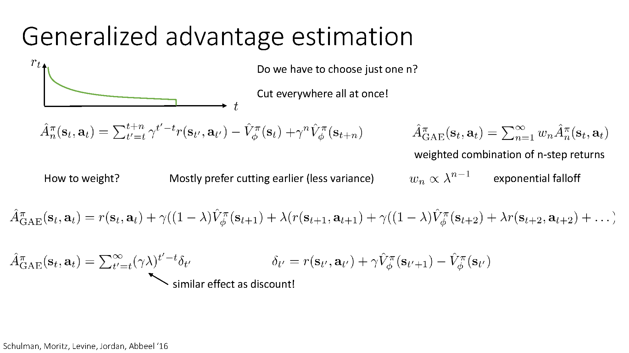
The parameter $\lambda$ controls estimator trust:

• $\lambda=0$: one-step TD; strongest bootstrapping, usually lowest variance;
• $\lambda\to1$: approaches Monte Carlo advantage on a complete trajectory; weaker critic bias, usually higher variance;
• between them: a smooth bias-variance tradeoff.

$\gamma$ changes what future reward means; $\lambda$ changes how that return is estimated. They appear together as $\gamma\lambda$, but they are not interchangeable.

PyTorch implementation

This implementation works backward through $N$ on-policy trajectories of horizon $H$. The code names values, deltas, and advantages correspond to $\hat V_\phi^\pi$, $\delta_t$, and $\hat A_{\mathrm{GAE}}^\pi$. Set the final next_values entry to zero for a terminal state, matching $\hat V_\phi^\pi(s_{H+1})=0$.

gae.py

import torch


@torch.no_grad()
def compute_gae(
    rewards: torch.Tensor,
    values: torch.Tensor,
    next_values: torch.Tensor,
    gamma: float = 0.99,
    gae_lambda: float = 0.95,
):
    """All tensors have shape [N, H]."""
    deltas = rewards + gamma * next_values - values

    advantages = torch.zeros_like(rewards)
    running_advantage = torch.zeros_like(rewards[:, 0])

    for t in range(rewards.shape[1] - 1, -1, -1):
        running_advantage = (
            deltas[:, t]
            + gamma
            * gae_lambda
            * running_advantage
        )
        advantages[:, t] = running_advantage

    value_targets = advantages + values
    return advantages, value_targets

Use the advantages as fixed actor weights and the value targets as fixed critic labels. The example assumes actor(states) returns a distribution whose log_prob(actions) has shape [N, H]; for vector-valued continuous actions, sum the per-dimension log-probabilities first.

actor_critic_update.py

values = critic(states).squeeze(-1)

with torch.no_grad():
    next_values = critic(next_states).squeeze(-1)
    advantages, value_targets = compute_gae(
        rewards,
        values.detach(),
        next_values,
        gamma=0.99,
        gae_lambda=0.95,
    )
    advantages = (advantages - advantages.mean()) / (
        advantages.std(unbiased=False) + 1e-8
    )

distribution = actor(states)
log_probs = distribution.log_prob(actions)

actor_loss = -(log_probs * advantages).mean()
critic_loss = 0.5 * (values - value_targets).square().mean()

actor_optimizer.zero_grad()
actor_loss.backward()
actor_optimizer.step()

critic_optimizer.zero_grad()
critic_loss.backward()
critic_optimizer.step()

Advantage normalization is an optimization heuristic: centering removes batch-wide offset and scaling makes the step size less sensitive to reward magnitude. GAE supplies the credit signal; algorithms such as PPO add another mechanism for controlling how far the policy may move.

Why replay breaks the on-policy derivation

Suppose the replay buffer $\mathcal R$ contains transitions generated by an older policy $\bar\pi$. Naively reusing stored actions creates two mismatches:

1. A $V^\pi$ Bellman target averages over actions from the current policy, but the stored action came from $\bar\pi$.
2. The policy-gradient sample also requires $a\sim\pi_\theta(a\mid s)$; inserting a stored $a\sim\bar\pi(a\mid s)$ is not the same estimator.

The key repair is to learn $Q(s,a)$, because it conditions on the stored action instead of averaging that action away.

For a replay batch ${(s_i,a_i,s_i’)}_{i=1}^{B}$, use the target from the lecture:

$$ y_i =r(s_i,a_i) +\gamma \mathbb{E}_{a_i'\sim\pi_\theta(a_i'\mid s_i')} [\hat Q_\phi^\pi(s_i',a_i')], $$

and fit

$$ \mathcal L(\phi) =\frac{1}{2}\sum_{i=1}^{B} \left\| \hat Q_\phi^\pi(s_i,a_i) -\operatorname{sg}(y_i) \right\|^2. $$

The old action $a_i$ is valid on the left because $Q$ is conditioned on it. The next action $a_i’$ must be freshly sampled from the latest policy because the target is evaluating that policy.

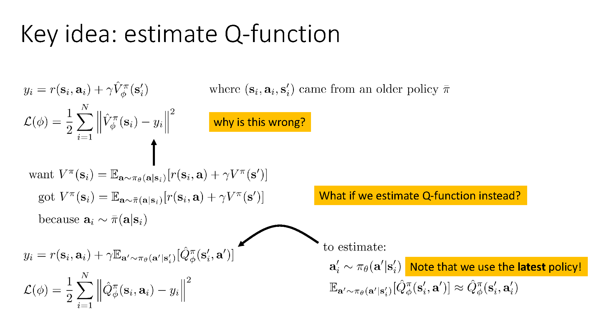
The actor also samples a fresh action at each replay state:

$$ \nabla_\theta J(\theta) \approx \frac{1}{N}\sum_{i=1}^{N} \nabla_\theta\log\pi_\theta(a_i^\pi\mid s_i) \hat Q_\phi^\pi(s_i,a_i^\pi), \qquad a_i^\pi\sim\pi_\theta(a_i^\pi\mid s_i). $$

This preserves the slide’s formula. In a score-function implementation, $\hat Q_\phi^\pi$ is held fixed during this actor step, just as the sampled weights were in Lecture 5; the slide does not write an explicit stop-gradient.

The replay states come from $\mathcal R$ rather than the current policy’s state marginal $p_\theta(s)$. Thus, despite the slide’s $\nabla_\theta J(\theta)$ label, this is generally a replay-distribution update direction rather than an unbiased gradient of the original on-policy objective. The slide describes the replay distribution intuitively as broader, but a real buffer may also have poor coverage. Reusing its data can improve sample efficiency; it does not guarantee it.

Reparameterization differentiates through the action

For the continuous Gaussian policy used in the lecture,

$$ \pi_\theta(a\mid s) =\mathcal N(\mu_\theta(s),\sigma_\theta(s)), \qquad \epsilon\sim\mathcal N(0,1), \qquad a=\mu_\theta(s)+\sigma_\theta(s)\epsilon. $$

Slide 32 uses this plus sign, while the algorithm on slide 33 shows a minus sign. The note keeps the sampling identity from slide 32. A symmetric Gaussian noise variable makes the two samples equal in distribution, but the plus sign keeps the computation consistent from sampling through differentiation.

The randomness now lives in $\epsilon$, whose distribution does not depend on $\theta$. Therefore

$$ \mathbb{E}_{a\sim\pi_\theta(a\mid s)}[Q(s,a)] =\mathbb{E}_{\epsilon\sim\mathcal N(0,1)} \left[ Q(s,\mu_\theta(s)+\sigma_\theta(s)\epsilon) \right] $$

can be differentiated directly through the action:

$$ \nabla_\theta J(\theta) \approx \sum_i \nabla_\theta \hat Q_\phi^\pi \left( s_i, \mu_\theta(s_i)+\sigma_\theta(s_i)\epsilon_i \right), \qquad \epsilon_i\sim\mathcal N(0,1). $$

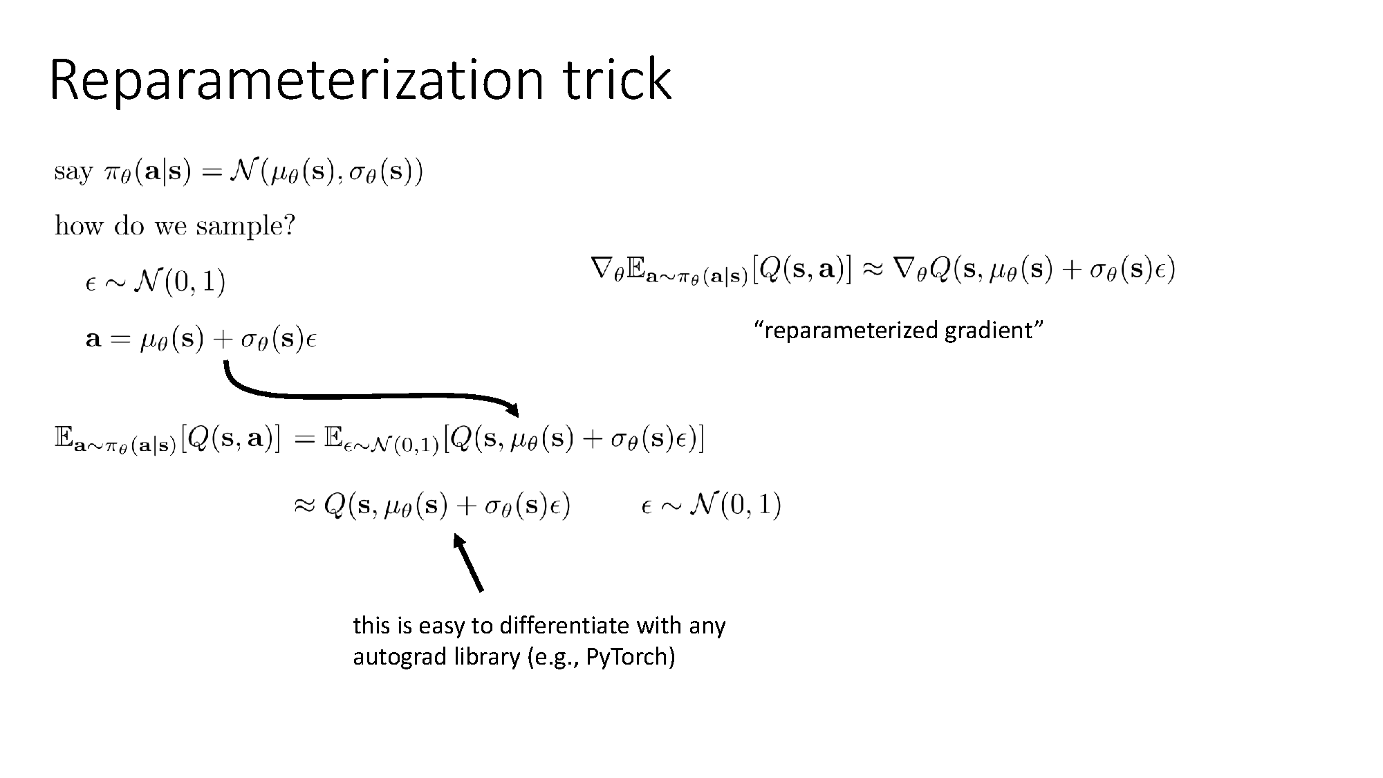
During the actor update, $\phi$ is fixed, but gradients flow through $\hat Q_\phi^\pi$ with respect to its action input. This reparameterized gradient is convenient for continuous actions and often has lower variance than the score-function estimator. Soft actor-critic builds on this idea, together with stronger Q-learning machinery and entropy regularization.

Common confusions

• Does the critic give rewards? No. Rewards come from the environment; the critic predicts expected return from those rewards.
• Is a critic an environment model? No. It predicts a scalar value, not the next state or full dynamics.
• Is $\delta_t$ exactly the advantage? Only in conditional expectation when the value function is exact. With an approximate critic it is an estimator.
• Does any inaccurate baseline bias policy gradient? A state-only baseline subtracted from Monte Carlo return does not. Bias enters when an inaccurate value is used to replace unobserved future rewards through bootstrapping.
• Are $\gamma$ and $\lambda$ the same kind of discount? No. $\gamma$ belongs to the return objective; $\lambda$ belongs to the advantage estimator.
• Can stored actions be inserted directly into an ordinary policy gradient? Not without an off-policy correction. Replay-based actor-critic instead conditions the critic on stored actions and samples fresh actor actions.

My takeaway

Actor-critic is easiest to understand as a credit-estimation system. The actor update itself barely changes; most of the design work goes into deciding what number should multiply $\nabla\log\pi$.

Monte Carlo return is honest but noisy. Bootstrapping is quieter but trusts an imperfect critic. GAE exposes this as a continuous choice rather than a binary one. Off-policy actor-critic makes a second trade: it gives up the exact current-policy state distribution so that experience can be reused, and a learned $Q(s,a)$ makes that reuse possible.

References

• Berkeley CS285 Lecture 6: Actor-Critic
• Schulman et al., High-Dimensional Continuous Control Using Generalized Advantage Estimation