CS285 DRL Notes-Lecture 4 Reinforcement Learning Basics

This is the note of Berkeley CS285, taught by Sergey Levine. Lecture 4 can be understood through one idea:

A policy is good only if the future state distribution it creates leads to high reward.

The whole RL problem in one loop

At every step,

s_t \xrightarrow{\pi_\theta(a_t\mid s_t)} a_t \xrightarrow{p(s_{t+1}\mid s_t,a_t)} (r(s_t,a_t),s_{t+1}).

The policy chooses an action; the environment returns a reward and the next state. An action matters through both its immediate reward and the future it creates.

Markov Decision Process

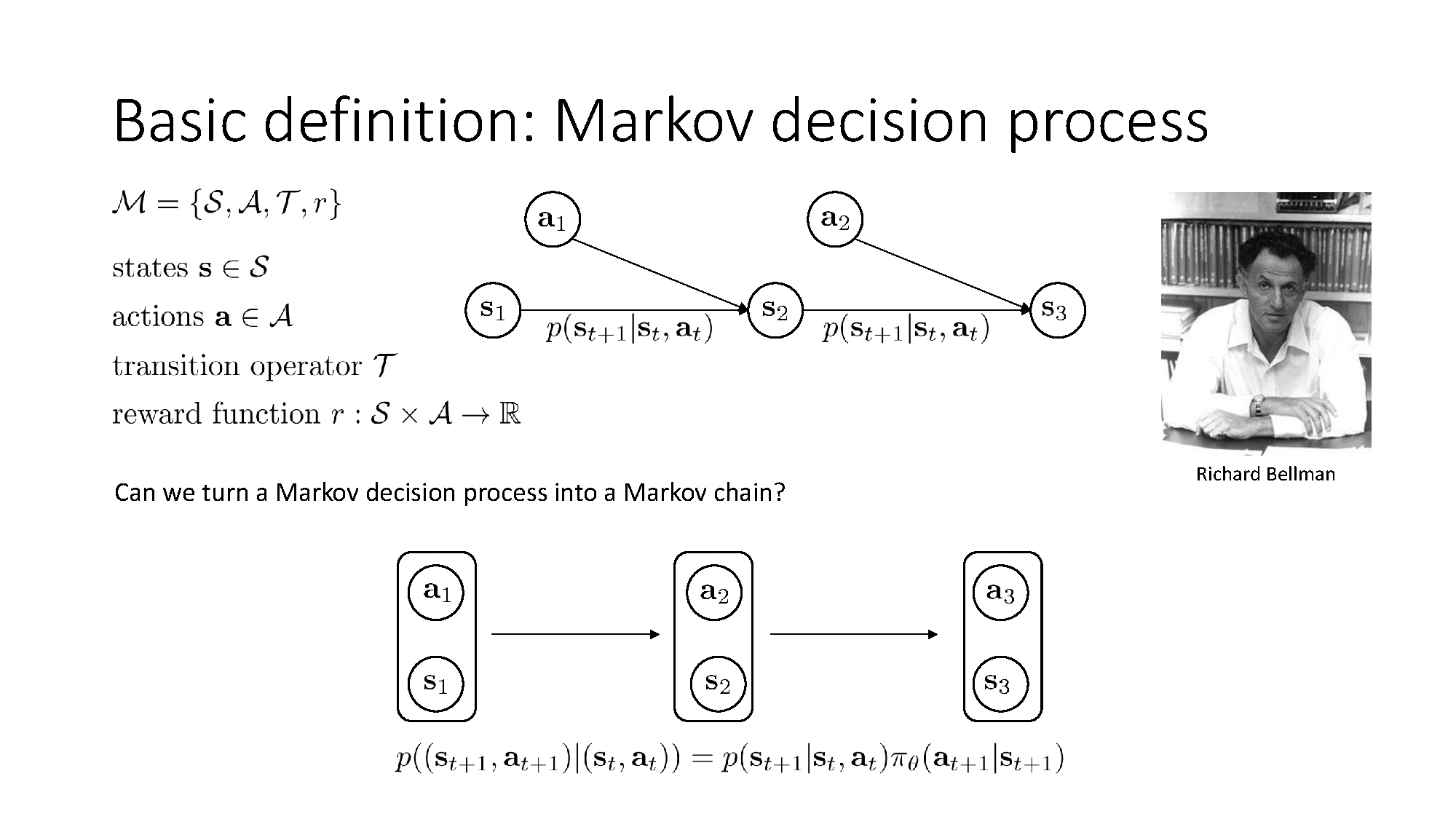
The lecture defines an MDP as

\mathcal M=\{\mathcal S,\mathcal A,\mathcal T,r\},

where $\mathcal T$ is the transition operator; the slides write its conditional probability or density as $p(s_{t+1}\mid s_t,a_t)$. A finite-horizon problem also needs the initial-state distribution $p(s_1)$ and horizon $H$, which are implicit in this compact definition. Infinite-horizon problems use either a discount $\gamma<1$ or a long-run average-reward objective.

The Markov property is

p(s_{t+1}\mid s_{1:t},a_{1:t}) =p(s_{t+1}\mid s_t,a_t).

This does not mean history is useless. It means $s_t$ already contains the relevant history.

If an observation $o_t$ hides relevant information, the problem is a POMDP and the agent needs memory or a belief state.

A policy creates a distribution over futures

Let a complete trajectory be

\tau=(s_1,a_1,\ldots,s_H,a_H,s_{H+1}).

The probability of this trajectory is

p_\theta(\tau) =p(s_1)\prod_{t=1}^{H} \pi_\theta(a_t\mid s_t) p(s_{t+1}\mid s_t,a_t).

This is the probability chain rule: the policy supplies action probabilities and the environment supplies transition probabilities.

The slide abbreviates the left side as $p_\theta(s_1,a_1,\ldots,s_H,a_H)$. Because its product includes the transition to $s_{H+1}$, the trajectory above writes that final state explicitly.

Trajectory Distribution

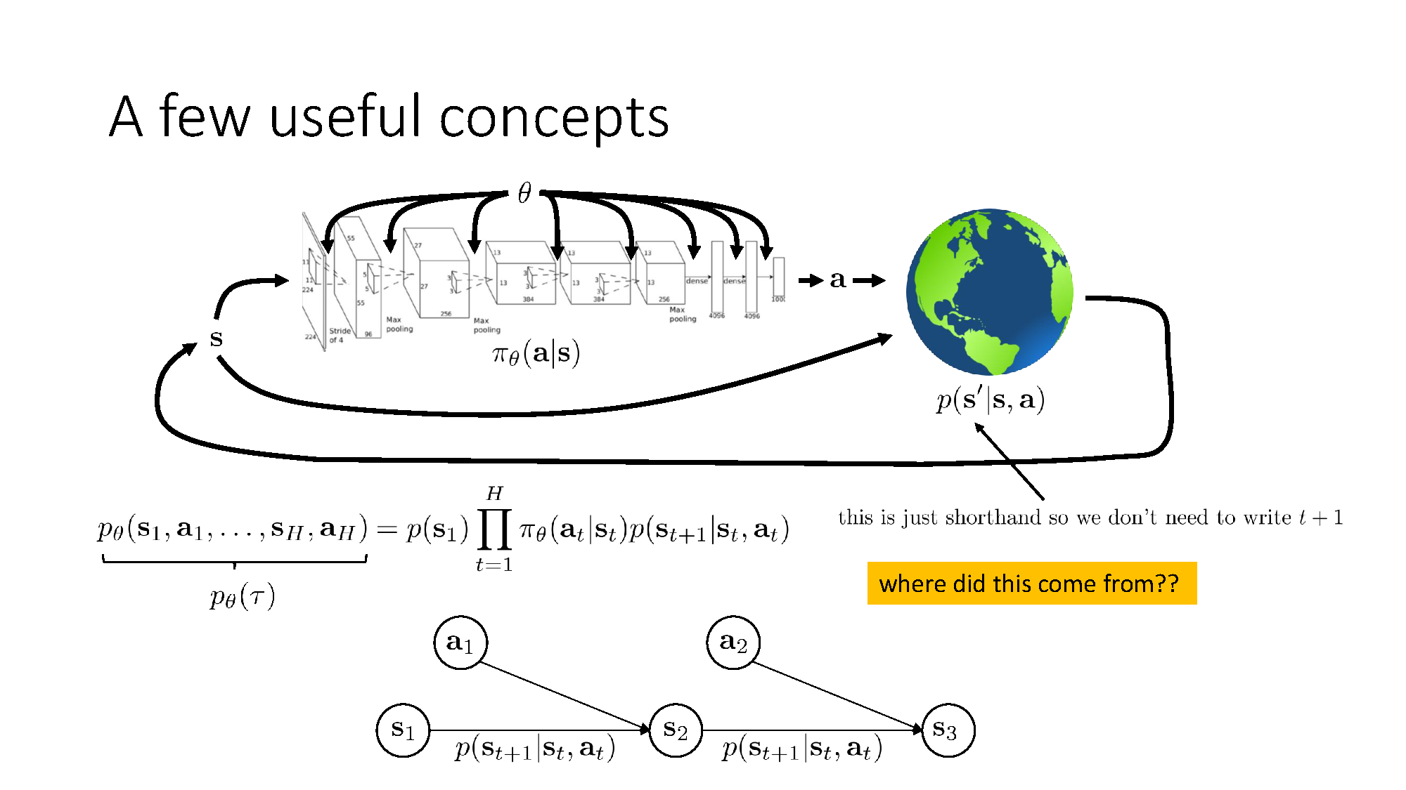
Although $\theta$ appears only in $\pi_\theta$, changing it also changes later states. RL therefore does not learn on a fixed input distribution.

State marginal

The slides denote the state marginal by $p_\theta(s_t)$. It is the trajectory distribution with every variable except $s_t$ summed out:

p_\theta(s_t) =\sum_{\mathbf a_{1:t-1},\mathbf s_{1:t-1}} p(s_1)\prod_{t'=1}^{t-1} \pi_\theta(a_{t'}\mid s_{t'}) p(s_{t'+1}\mid s_{t'},a_{t'}).

For discrete states this is a probability mass; for continuous states it is a density, and the sums become integrals. The state-action marginal is

p_\theta(s_t,a_t) =p_\theta(s_t)\pi_\theta(a_t\mid s_t).

The trajectory distribution describes complete futures; $p_\theta(s_t)$ is one projection of it. Once $\pi_\theta$ is fixed, the MDP becomes a Markov chain. Its stationary distribution, when it exists, describes where the policy spends time in the long run.

The objective is reward under that distribution

The lecture’s finite-horizon objective is

\theta^\star =\arg\max_\theta \mathbb E_{\tau\sim p_\theta(\tau)} \left[\sum_t r(s_t,a_t)\right].

Call the expectation on the right $J(\theta)$. The lecture is undiscounted here; a discounted objective inserts $\gamma^{t-1}$ without changing the distributional idea.

RL Objective

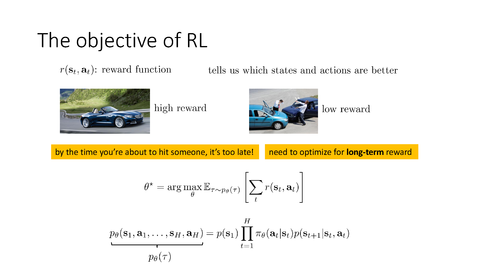
Using state-action marginals, the same objective is

J(\theta) =\sum_{t=1}^{H} \mathbb E_{(s_t,a_t)\sim p_\theta(s_t,a_t)} [r(s_t,a_t)].

Changing $\theta$ changes both action probabilities and the future data distribution $p_\theta(s_t,a_t)$. Reward evaluates one step; the sum evaluates the future. RL must assign later reward to earlier actions.

If $p_\theta(s_t,a_t)$ converges to the slide’s stationary distribution $\bar\mu$, the long-run average reward is $\mathbb E_{(s,a)\sim\bar\mu}[r(s,a)]$.

V and Q are conditional versions of the same objective

The Q-function fixes the current state and action, then averages the remaining rewards under the policy:

Q^\pi(s_t,a_t) =\sum_{t'=t}^{T} \mathbb E_{\pi_\theta} [r(s_{t'},a_{t'})\mid s_t,a_t].

The value function fixes only the current state:

V^\pi(s_t) =\sum_{t'=t}^{T} \mathbb E_{\pi_\theta} [r(s_{t'},a_{t'})\mid s_t].

After the first action, both follow $\pi_\theta$. Thus, $Q^\pi(s_t,a_t)$ measures the long-term consequence of choosing $a_t$ now.

They satisfy

V^\pi(s_t) =\mathbb E_{a_t\sim\pi_\theta(a_t\mid s_t)}[Q^\pi(s_t,a_t)],

and the original objective is simply

J(\theta)=\mathbb E_{s_1\sim p(s_1)}[V^\pi(s_1)].

Value Functions

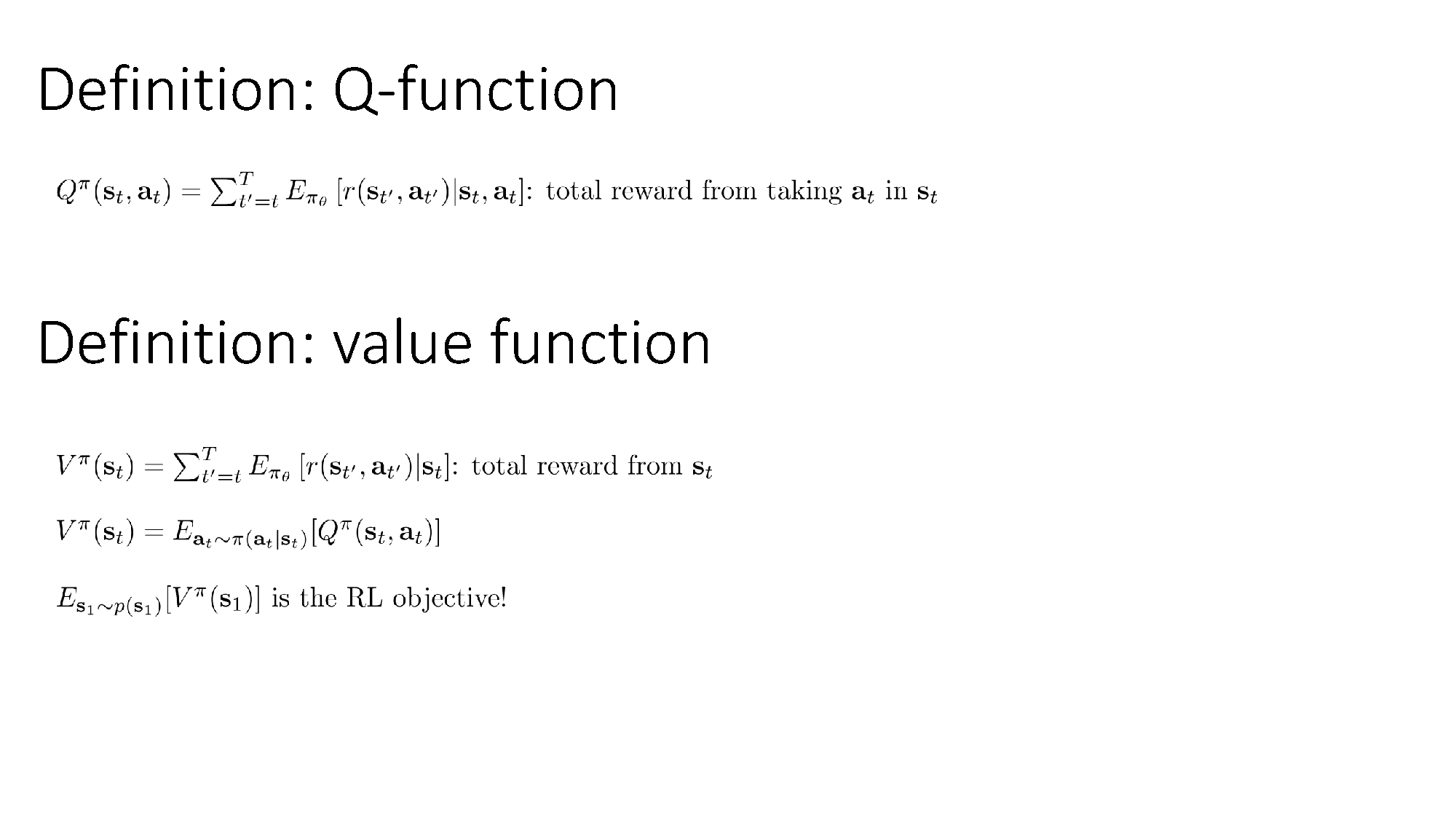
The key interpretation is: $J$ is the global objective; $V$ and $Q$ are the same objective conditioned on where we are and what we do next. The slides keep time in the arguments $s_t,a_t$ but omit it from the function names. In a finite horizon, value generally depends on time unless time is included in the state.

Bellman equation: now plus later

Separating the first reward from the remaining return gives the Bellman equation:

Q^\pi(s_t,a_t) =r(s_t,a_t) +\mathbb E_{s_{t+1}\sim p(s_{t+1}\mid s_t,a_t)} [V^\pi(s_{t+1})],

V^\pi(s_t) =\mathbb E_{a_t\sim\pi_\theta(a_t\mid s_t)}[Q^\pi(s_t,a_t)], \qquad V^\pi(s_{T+1})=0.

It is an identity, not a new objective or an algorithm. Algorithms differ in how they estimate it from data. In a discounted formulation, the future-value term is multiplied by $\gamma$.

The advantage function is

A^\pi(s_t,a_t)=Q^\pi(s_t,a_t)-V^\pi(s_t).

Advantage asks whether $a_t$ is better than the policy’s average action at $s_t$. A basic policy-improvement rule increases the probability of actions with positive advantage.

One question unifies RL algorithms

Every RL algorithm must answer one counterfactual: what would happen if the agent chose a different action?

Types of RL Algorithms

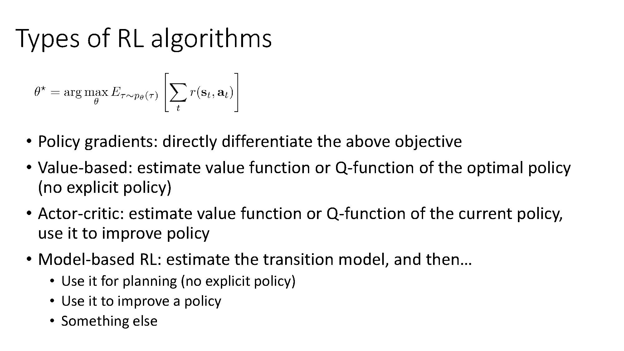
Method	What it estimates or learns	How it improves behavior	Main difficulty
Policy gradient	$\nabla_\theta J(\theta)$	Changes action probabilities directly	Noisy gradient estimates
Value-based	$V$ or $Q$, often for the optimal policy	Chooses actions with high estimated value	Bootstrapping and value errors
Actor-critic	A policy plus $V$, $Q$, or $A$ for that policy	Uses the critic to update the actor	Bias-variance and coupled training
Model-based	The transition model, plus a reward model when reward is unknown	Predicts outcomes and plans through them	Model error compounds during planning

Most methods still repeat the same loop:

Collect experience.
Estimate future consequences.
Change the policy.

They differ mainly in whether sampled returns, a value function, or a model represents the future.

Sample efficiency and stability

Environment interaction is often the real cost.

On-policy: data matches the current policy, but old data quickly becomes less useful.
Off-policy: data can be reused across policies, but distribution mismatch complicates learning.
Model-based: imagined data is cheap, but only as reliable as the model.

Sample Efficiency

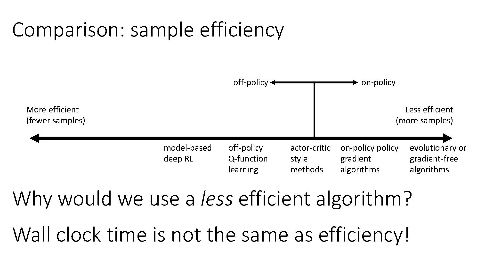
The figure shows a tendency, not a universal ranking. Reusing more samples does not guarantee faster or more stable learning.

Model learning minimizes prediction error, value learning often minimizes Bellman error, and exact policy gradient differentiates $J$. None is automatically stable once data, function approximation, and sampling error enter.

Common confusions

Reward is not Q-value. Reward is immediate; Q-value includes the future.
A model is not a policy. The model predicts what the environment will do; the policy chooses what the agent will do.
State marginal is not trajectory distribution. It keeps one state and removes the other trajectory variables.
Bellman equation is not the RL objective. It is a recursive identity satisfied by value functions.
Model-free does not mean the world has no dynamics. It means the agent does not plan with an explicit learned dynamics model.

My takeaway

A policy matters because it changes future state distributions, not just current actions.
$J$ is expected return; $V$, $Q$, and advantage are local views of that same objective.
RL families differ mainly in how they estimate the consequences of alternative actions.
Algorithm choice is a tradeoff among data reuse, estimation error, model bias, stability, and interaction cost.