CS285 DRL Notes-Lecture 5 Policy Gradients

This is the note for Berkeley CS285 Lecture 5. The lecture introduces the simplest model-free policy-gradient method: REINFORCE.

The central idea is simple: make sampled actions more likely when their outcomes are better than expected, and less likely when their outcomes are worse than expected.

From expected return to a policy gradient

For a trajectory

$$ \tau=(s_1,a_1,\ldots,s_H,a_H,s_{H+1}), $$

define its return as

$$ r(\tau)=\sum_{t=1}^{H}r(s_t,a_t). $$

The policy induces the trajectory distribution

$$ p_\theta(\tau) =p(s_1)\prod_{t=1}^{H}\pi_\theta(a_t\mid s_t) p(s_{t+1}\mid s_t,a_t), $$

and the RL objective is

$$ J(\theta)=\mathbb{E}_{\tau\sim p_\theta(\tau)}[r(\tau)]. $$

The difficulty is that $\theta$ changes the distribution we sample from. The log-derivative identity turns this into an ordinary expectation:

$$ \begin{aligned} \nabla_\theta J(\theta) &=\int \nabla_\theta p_\theta(\tau)r(\tau)d\tau\\ &=\int p_\theta(\tau)\nabla_\theta\log p_\theta(\tau)r(\tau)d\tau\\ &=\mathbb{E}_{\tau\sim p_\theta} \left[\nabla_\theta\log p_\theta(\tau)r(\tau)\right]. \end{aligned} $$

Assuming the initial-state distribution and environment dynamics do not depend on $\theta$,

$$ \nabla_\theta\log p_\theta(\tau) =\sum_{t=1}^{H}\nabla_\theta\log\pi_\theta(a_t\mid s_t). $$

Therefore,

$$ \nabla_\theta J(\theta) =\mathbb{E}_{\tau\sim p_\theta} \left[ \left(\sum_{t=1}^{H}\nabla_\theta\log\pi_\theta(a_t\mid s_t)\right) r(\tau) \right]. $$

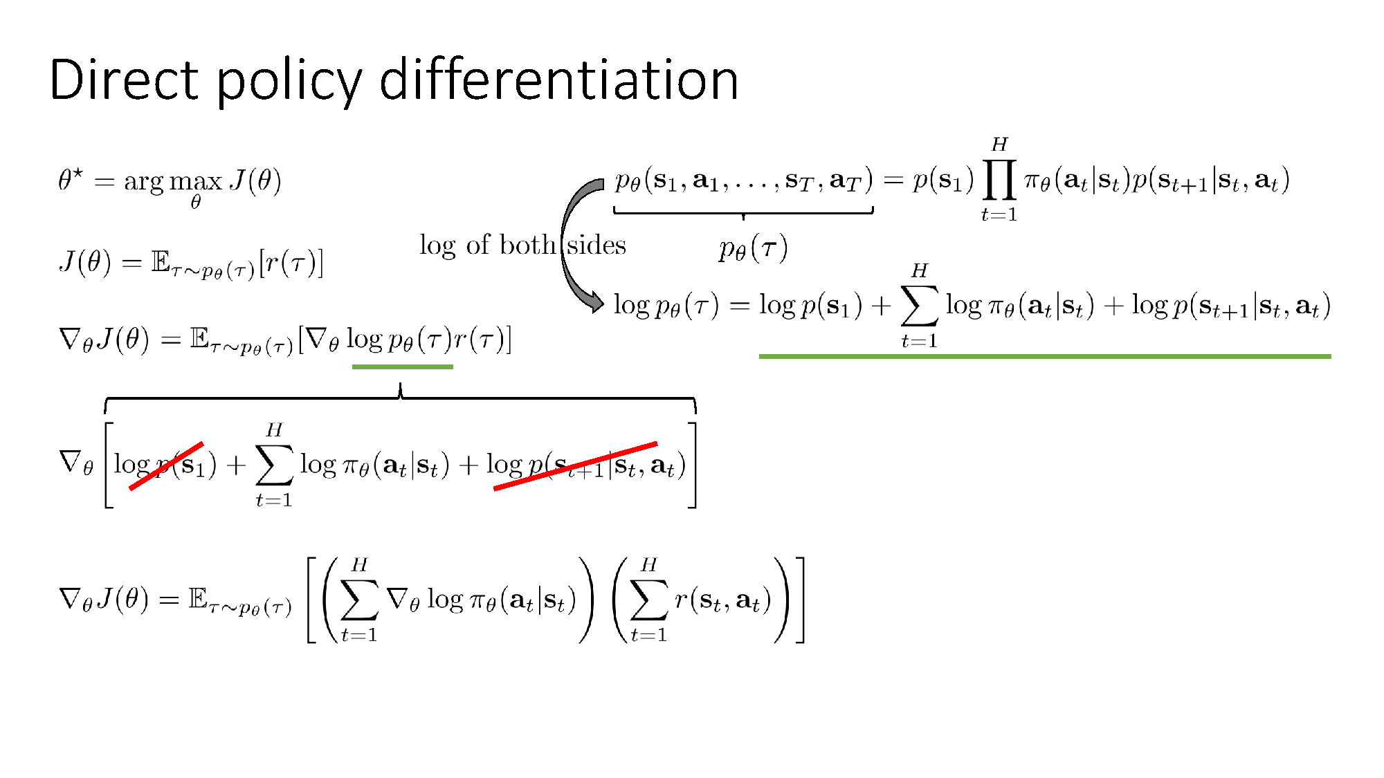
The source image mixes $T$ and $H$ and abbreviates the trajectory before the final state. The equations above use one horizon symbol $H$ and include $s_{H+1}$ because the product contains the final transition.

This is the key trick: we do not differentiate through the environment. We only need sampled rewards and the gradient of the policy’s log-probability.

The derivation also does not require the policy input to be a Markov state. Replacing $s_t$ with an observation or history gives the same estimator, so policy gradients also apply to partially observed environments.

REINFORCE as reward-weighted maximum likelihood

With $N$ sampled trajectories, REINFORCE estimates the gradient by

$$ \nabla_\theta J(\theta) \approx\frac{1}{N}\sum_{i=1}^{N} \left(\sum_{t=1}^{H}\nabla_\theta \log\pi_\theta(a_t^{(i)}\mid s_t^{(i)})\right)r(\tau^{(i)}). $$

Maximum likelihood increases the log-probability of every action in a fixed dataset. REINFORCE has the same gradient shape, but each sampled trajectory is weighted by its return:

• positive weight: make its actions more likely;
• negative weight: make its actions less likely;
• larger magnitude: make a larger update.

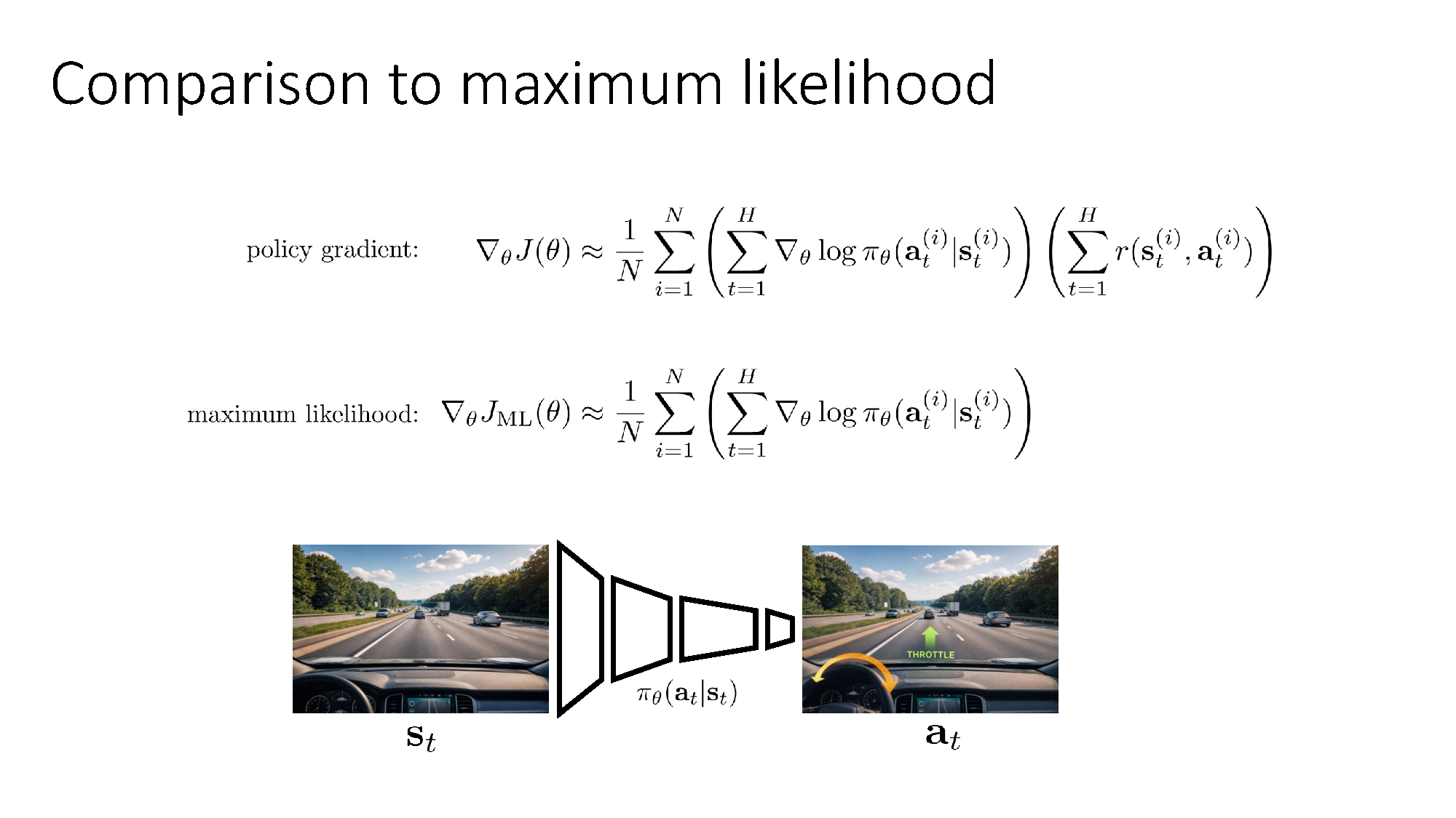
The similarity is useful, but the two objectives are not the same. Maximum likelihood imitates fixed target actions. REINFORCE collects actions from the current policy and receives their weights from the environment.

For the slide’s Gaussian example, write the neural-network mean as $f_\theta(s)$ and let $\pi_\theta(a\mid s)=\mathcal N(f_\theta(s),\Sigma)$ with fixed covariance. The corrected score is

$$ \nabla_\theta\log\pi_\theta(a\mid s) =\left(\frac{\partial f_\theta(s)}{\partial\theta}\right)^\top \Sigma^{-1}(a-f_\theta(s)). $$

So a positive return moves the mean toward the sampled action, while a negative return moves it away. Slide 11’s displayed derivative loses factors when differentiating the quadratic log-density; the expression above is the minimal correction while retaining its $f$ notation.

Why the naive estimator is noisy

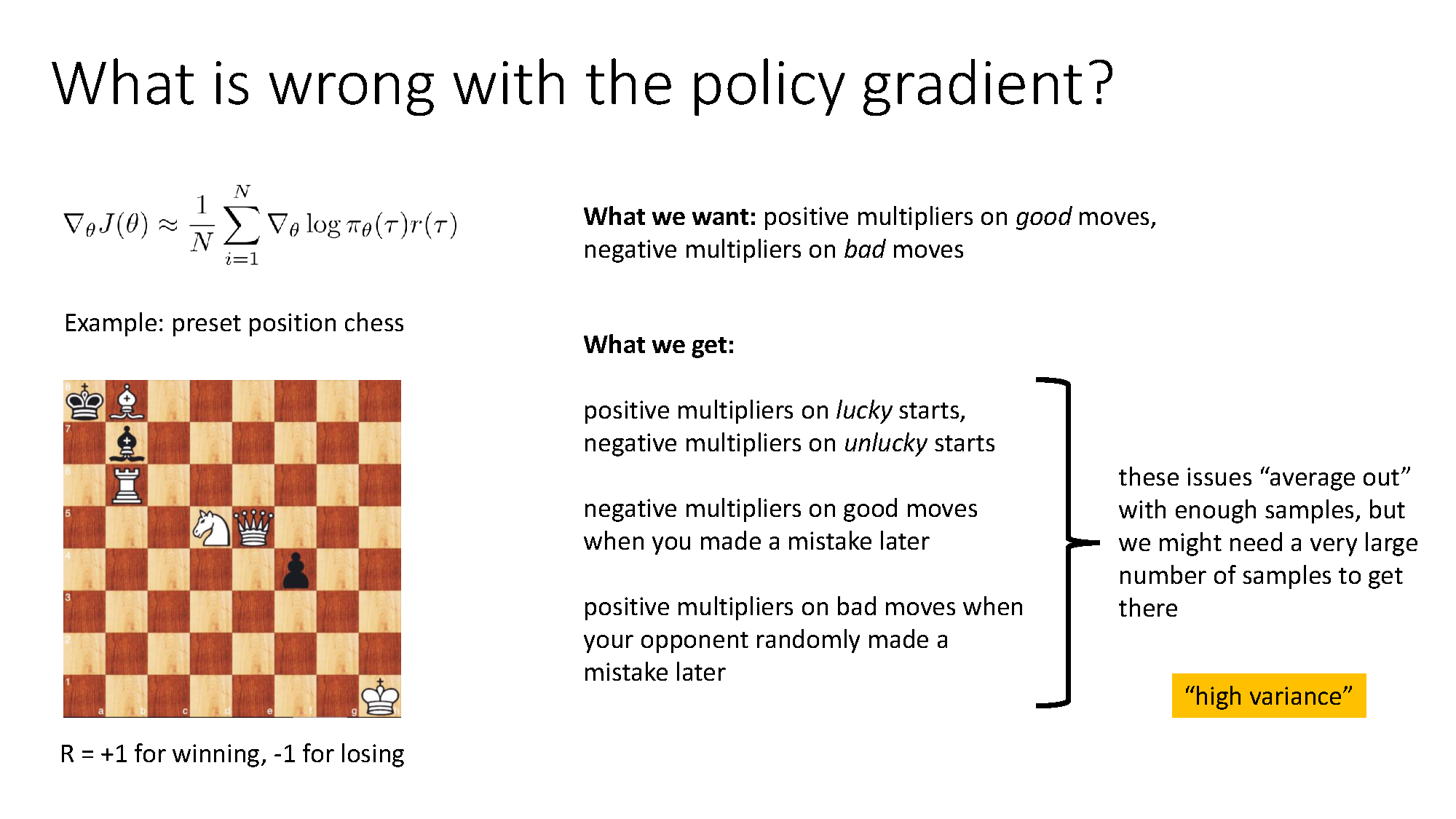
The first estimator gives the same total return to every action in a trajectory. This creates weak credit assignment:

• a good action can receive a negative weight because of a later mistake;
• a bad action can receive a positive weight because of later luck;
• even the starting state can change the return without being caused by the policy.

These errors cancel with enough samples, so the estimator is unbiased, but the number of samples may be very large. This is what high variance means here.

Two ideas remove noise without changing the expected gradient: baselines and causality.

Baselines remove irrelevant scale

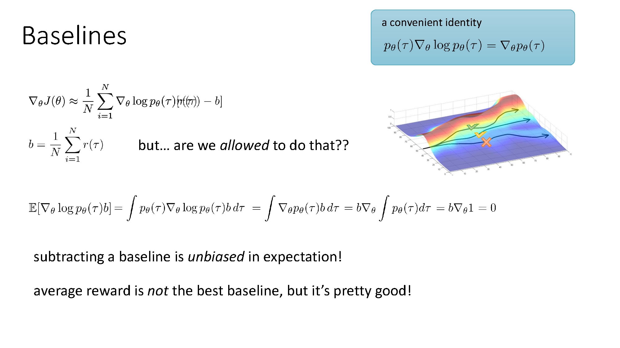
We may subtract a scalar baseline $b$ that does not depend on the sampled action:

$$ \begin{aligned} \mathbb{E}_{a_t\sim\pi_\theta(\cdot\mid s_t)} \left[\nabla_\theta\log\pi_\theta(a_t\mid s_t)b\right] &=b\nabla_\theta\int\pi_\theta(a_t\mid s_t)da_t\\ &=b\nabla_\theta 1=0. \end{aligned} $$

The baseline therefore changes the variance, not the expected gradient. A common choice is a running estimate of the mean return. It changes the question from “was the return positive?” to “was it better than the usual return?”

Causality gives reward-to-go

An action at time $t$ cannot affect rewards received before time $t$. Those past rewards are pure noise for that action’s gradient and can be removed. Define the reward-to-go

$$ G_t=\sum_{t'=t}^{H}r(s_{t'},a_{t'}). $$

With $N$ sampled trajectories, the lecture’s reward-to-go estimator is

$$ \nabla_\theta J(\theta) \approx\frac{1}{N}\sum_{i=1}^{N}\sum_{t=1}^{H} \nabla_\theta\log\pi_\theta(a_t^{(i)}\mid s_t^{(i)}) \hat Q_t^{(i)}. $$

Following the notation in the lecture slides, the baseline-subtracted Monte Carlo weight is

$$ \hat Q_t^{(i)} =\sum_{t'=t}^{H}r(s_{t'}^{(i)},a_{t'}^{(i)})-b =G_t^{(i)}-b. $$

This is the quantity called q_values in the original pseudocode. It measures whether the sampled future return was above or below the reference level $b$. Strictly speaking, it is a centered Monte Carlo estimate rather than the uncentered value $Q^\pi(s_t,a_t)$.

Reward-to-go removes rewards that the action could not possibly cause. It does not remove all future randomness, so policy-gradient estimation can still have high variance.

The pseudo-loss used in code

The lecture first introduces a scalar ascent surrogate whose gradient gives the sampled estimator:

$$ \widetilde J(\theta) \approx\frac{1}{N}\sum_{i=1}^{N}\sum_{t=1}^{H} \log\pi_\theta(a_t^{(i)}\mid s_t^{(i)}) \hat Q_t^{(i)}. $$

Most automatic-differentiation libraries minimize a loss, so the actual implementation uses

$$ L_{\mathrm{PG}}(\theta) =-\frac{1}{N}\sum_{i=1}^{N}\sum_{t=1}^{H} \log\pi_\theta(a_t^{(i)}\mid s_t^{(i)}) \operatorname{sg}\!\left(\hat Q_t^{(i)}\right). $$

The slide does not write $\operatorname{sg}$. It appears here to state the code semantics explicitly: during this actor update, sampled $\hat Q_t^{(i)}$ values are fixed weights. The minus sign converts ascent on $\widetilde J$ into descent on $L_{\mathrm{PG}}$.

PyTorch implementation

The following implementation assumes a discrete policy whose network returns action logits. states, actions, and rewards contain one on-policy batch with shapes [N, H, state_dim], [N, H], and [N, H].

First compute reward-to-go without constructing an autograd graph:

reward_to_go.py

import torch


@torch.no_grad()
def reward_to_go(rewards: torch.Tensor, gamma: float = 1.0) -> torch.Tensor:
    """Compute G_t for a fixed-horizon batch. rewards has shape [N, H]."""
    returns = torch.zeros_like(rewards)
    running_return = torch.zeros(
        rewards.shape[0], device=rewards.device, dtype=rewards.dtype
    )

    for t in range(rewards.shape[1] - 1, -1, -1):
        running_return = rewards[:, t] + gamma * running_return
        returns[:, t] = running_return

    return returns

Then use the sampled $\hat Q_t$ values as fixed weights in the policy update:

reinforce_update.py

from torch.distributions import Categorical


def reinforce_update(
    policy,
    optimizer,
    states: torch.Tensor,
    actions: torch.Tensor,
    rewards: torch.Tensor,
    b: torch.Tensor,
    gamma: float = 1.0,
):
    returns = reward_to_go(rewards, gamma)

    # sg(G_t - b): fixed weights for the actor update
    q_values = (returns - b).detach()

    logits = policy(states)
    distribution = Categorical(logits=logits)
    log_probs = distribution.log_prob(actions)

    # -(1/N) * sum_i sum_t log pi(a_t|s_t) * Q_t
    policy_loss = -(log_probs * q_values).sum(dim=1).mean()

    optimizer.zero_grad()
    policy_loss.backward()
    optimizer.step()

    # Use the full trajectory return to update b after the actor step.
    batch_mean_return = returns[:, 0].mean()
    return policy_loss.item(), batch_mean_return

Maintain the scalar baseline as a running mean:

training_step.py

b = torch.zeros((), device=device)
baseline_momentum = 0.9

# states, actions, rewards must come from fresh rollouts of the current policy.
loss_value, batch_mean_return = reinforce_update(
    policy, optimizer, states, actions, rewards, b
)

with torch.no_grad():
    b.mul_(baseline_momentum).add_(
        batch_mean_return, alpha=1.0 - baseline_momentum
    )

There are three important details:

1. Categorical(logits=logits) computes a numerically stable log-probability without applying softmax manually.
2. The minus sign converts gradient ascent on expected return into gradient descent on policy_loss.
3. q_values.detach() implements $\operatorname{sg}(\hat Q_t)$. For pure REINFORCE, environment returns normally have no gradient path, so this is redundant but explicit. Detaching is required only when the weight has a path to actor or shared parameters and this update is meant to implement the score-function surrogate. It is not used to cut the critic-to-action path in a reparameterized actor update.

For continuous actions, replace Categorical with a distribution such as Independent(Normal(mean, std), 1); the loss construction is unchanged.

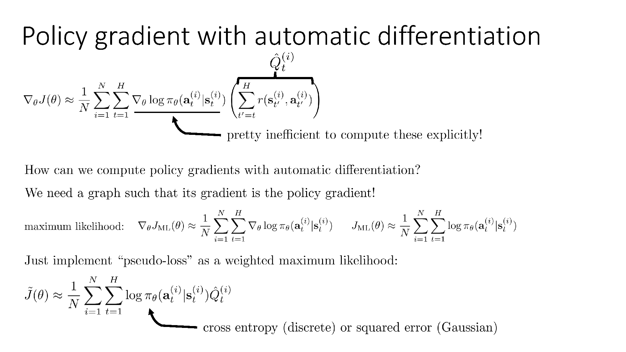
This is a surrogate for computing the gradient, not the original RL objective itself. The sampled q_values must be treated as fixed weights; otherwise autodiff would differentiate through quantities that the score-function derivation treats as samples.

The practical loop is short:

1. Run the current policy and collect fresh trajectories.
2. Compute each reward-to-go $G_t$.
3. Compute or update a scalar baseline and form $\hat Q_t=G_t-b$.
4. Minimize the pseudo-loss once with the on-policy batch.
5. Repeat with new data.

Larger batches usually stabilize REINFORCE, while larger learning rates make its noisy updates more dangerous.

Common confusions

• Where does the reward come from? The environment returns it after an action. REINFORCE only uses that reward to weight log-probability gradients.
• Is REINFORCE maximum likelihood? It uses the same log-likelihood machinery, but the data are on-policy and the weights are signed returns or baseline-subtracted $Q$ estimates.
• Does unbiased mean stable? No. The average direction can be correct while individual gradient estimates vary wildly.
• Does a baseline change the optimal policy? No, provided it is independent of the sampled action inside the score term.
• Is the pseudo-loss the expected return? No. Its gradient matches the estimator; its numerical value has no direct control meaning.

My takeaway

Policy gradient is best understood as credit-weighted imitation of the policy’s own experience. The policy samples actions, the environment judges the outcomes, and the log-probability gradient turns that judgment into an update.

The derivation is elegant; the real difficulty is statistical. Full-trajectory returns give correct but noisy credit. Reward-to-go removes causally impossible credit, and a baseline turns raw return into relative performance. That progression leads directly from REINFORCE to advantage-based actor-critic methods.

References

• Berkeley CS285: Deep Reinforcement Learning
• CS285 Lecture 5: Policy Gradients