CS285 DRL Notes-Lecture 2 Supervised Learning of Behaviors

This is the note of Berkeley CS285 taught by Sergey Levine. Lecture 2 studies the simplest way to learn a policy from an expert: behavioral cloning.

The central idea is easy to miss:

Behavioral cloning is ordinary supervised learning during training, but it is not ordinary supervised learning after deployment. The policy’s prediction changes the next input it will receive.

That feedback loop explains both the usefulness and the main weakness of imitation learning.

Behavioral cloning is maximum likelihood

Suppose an expert provides $N$ trajectories of length $H$:

\mathcal D=\{\tau^{(i)}\}_{i=1}^{N},\qquad \tau^{(i)}=(o_1^{(i)},a_1^{(i)},\ldots,o_H^{(i)},a_H^{(i)}).

Behavioral cloning (BC) treats every expert pair $(o_t,a_t)$ as a supervised example and fits the policy by maximum likelihood:

\arg\max_\theta \sum_{i=1}^{N}\sum_{t=1}^{H} \log \pi_\theta\!\left(a_t^{(i)}\mid o_t^{(i)}\right).

Equivalently, it minimizes negative log-likelihood. For discrete actions, the network usually outputs class probabilities. For continuous actions, it can output the parameters of a distribution such as a Gaussian.

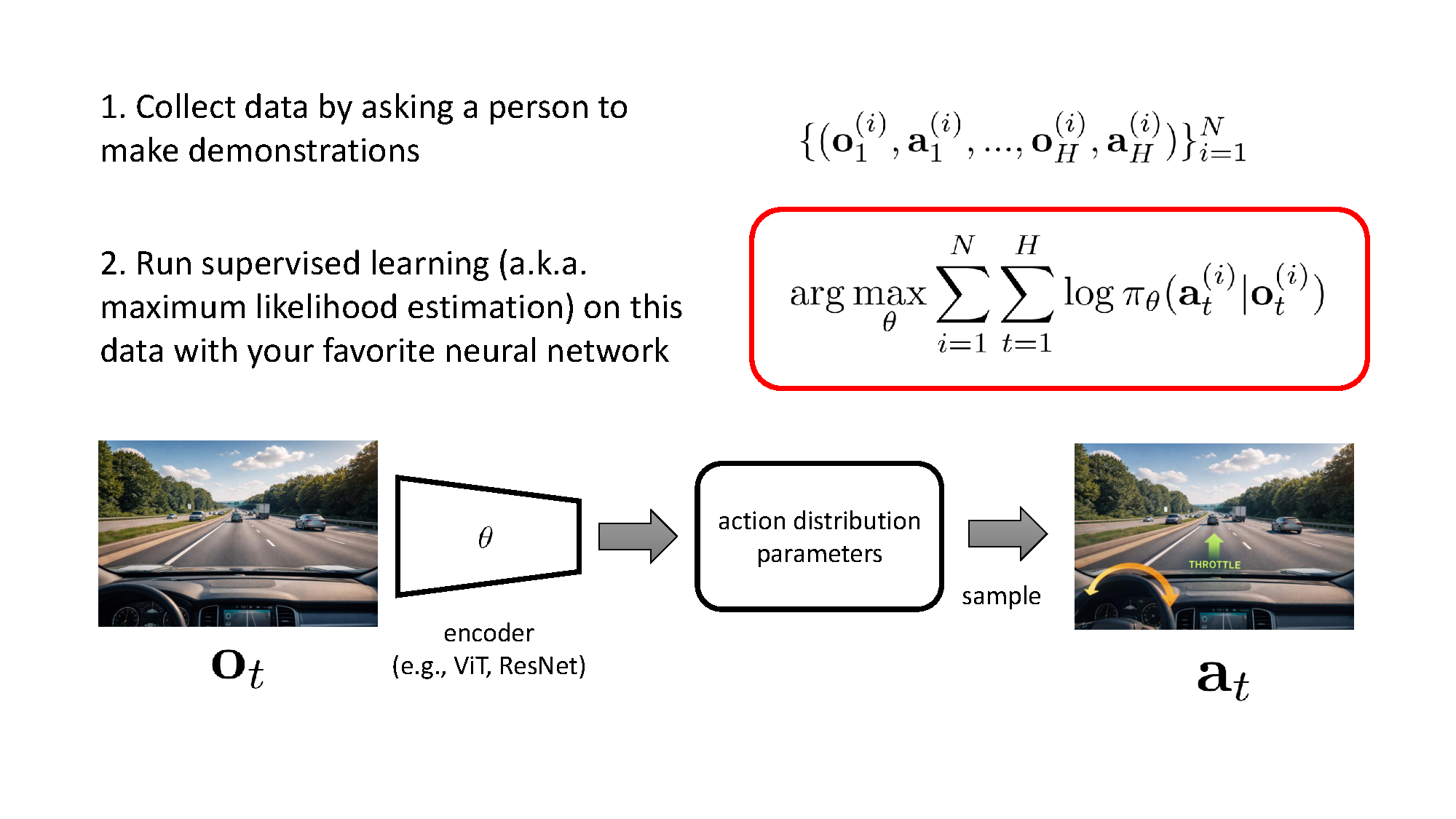
Behavioral cloning pipeline from expert demonstrations to a learned policy

The environment may have a hidden state $s_t$, an observation model $p(o_t\mid s_t)$, and dynamics $p(s_{t+1}\mid s_t,a_t)$. BC does not need to learn these models. It only needs expert input-action pairs. However, the dynamics still matter at deployment because every predicted action determines which states will be visited next.

Training accuracy is not rollout accuracy

The lecture writes the observation distribution in the demonstrations as $p_{\mathrm{data}}(o_t)$ and the distribution created by the learned policy as $p_{\pi_\theta}(o_t)$. BC optimizes log-likelihood under the first distribution, but the policy is evaluated under the second.

An early steering mistake, for example, moves the car away from the expert’s trajectory. The next image is then an image the model may never have seen in training. The policy is no longer merely making another independent prediction; it is predicting on data created by its previous predictions.

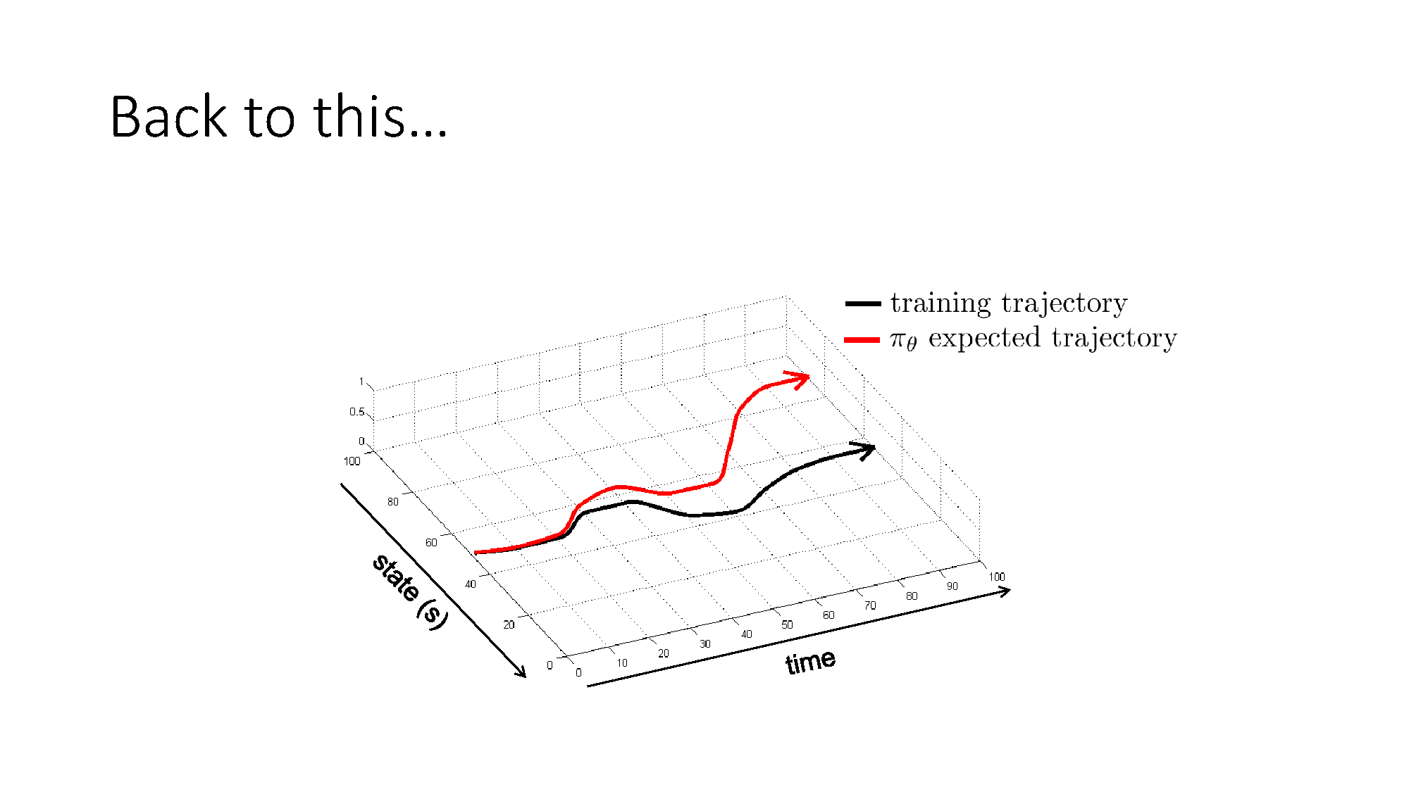
A small policy error moves the learner away from the expert state distribution

This is distributional shift in imitation learning:

p_{\mathrm{data}}(o_t)\neq p_{\pi_\theta}(o_t).

The key distinction is therefore:

A small supervised loss says the policy imitates the expert well where the expert goes.
A good controller must act well where the policy itself goes.

Why a small error can grow with the horizon

For the theoretical argument, the slides switch to a fully observed state and define the one-step mistake cost

c(s_t,a_t)= \begin{cases} 0,&a_t=\pi^\star(s_t),\\ 1,&\text{otherwise}, \end{cases} \qquad \mathbb E_{a_t\sim\pi_\theta(a_t\mid s_t)}[c(s_t,a_t)] =\pi_\theta(a_t\neq\pi^\star(s_t)\mid s_t).

The expected total number of rollout mistakes is therefore

\sum_{t=1}^{H} \mathbb E_{\substack{a_t\sim\pi_\theta(a_t\mid s_t)\\ s_t\sim p_{\pi_\theta}(s_t)}} [c(s_t,a_t)].

Assume the policy’s mistake probability under the training-state distribution is at most $\epsilon$:

\mathbb E_{s_t\sim p_{\mathrm{train}}(s_t)} [\pi_\theta(a_t\neq\pi^\star(s_t)\mid s_t)] \leq\epsilon.

Before the first mistake, learner and expert can be coupled to follow the same trajectory. The slides express the resulting state distribution as

p_{\pi_\theta}(s_t) =(1-\epsilon)^t p_{\mathrm{train}}(s_t) +\left(1-(1-\epsilon)^t\right)p_{\mathrm{mistake}}(s_t).

Hence the total-variation gap can grow linearly with time,

D_{\mathrm{TV}}\!\left(p_{\mathrm{train}},p_{\pi_\theta}\right) \leq 1-(1-\epsilon)^t \leq\epsilon t,

and the slide’s final bound is

\sum_{t=1}^{H} \mathbb E_{\substack{a_t\sim\pi_\theta(a_t\mid s_t)\\ s_t\sim p_{\pi_\theta}(s_t)}}[c(s_t,a_t)] \leq\sum_{t=1}^{H}(\epsilon+2\epsilon t) =O(\epsilon H^2).

The factor 2 comes from $\lVert p-q\rVert_1=2D_{\mathrm{TV}}(p,q)$. The slides count the bound with $t$; if $s_t$ is defined after exactly $t-1$ previous actions, the corresponding factors become $t-1$. This indexing change does not alter the $O(\epsilon H^2)$ conclusion.

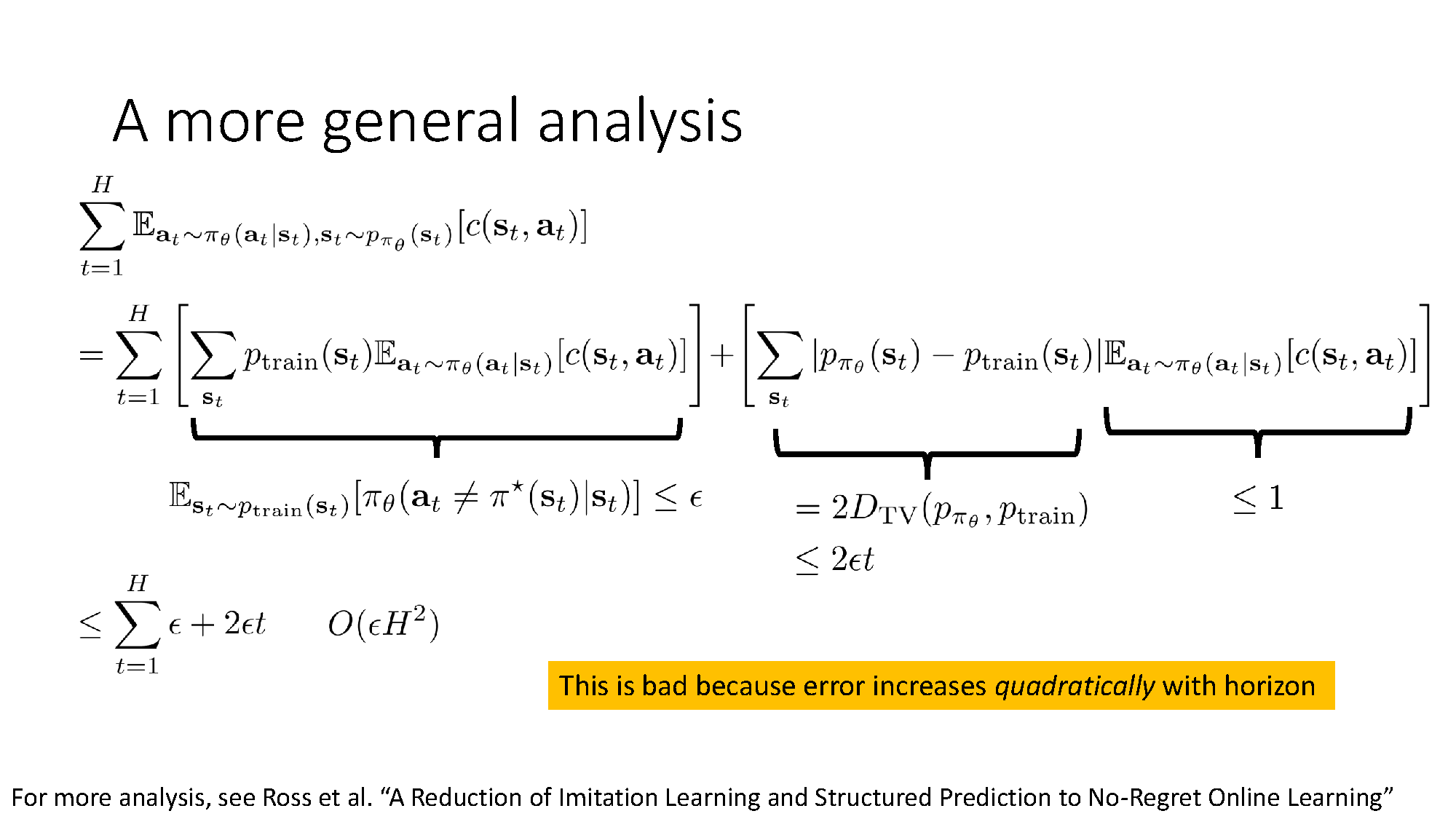
Worst-case behavioral-cloning error grows quadratically with the horizon

This is a worst-case bound, not a prediction that every BC policy must fail quadratically. It says that a low one-step error alone is insufficient to guarantee a good long rollout.

Why behavioral cloning can still work

BC can work well when at least one of the following is true:

The policy’s one-step error $\epsilon$ is extremely small.
The system naturally returns toward the expert trajectory.
The demonstration data includes off-center states and recovery actions.
Data augmentation creates realistic correction examples.

The driving example in the lecture uses side cameras and corrected steering labels. This is not merely “more data.” It teaches the policy what to do after it has drifted away from the nominal trajectory.

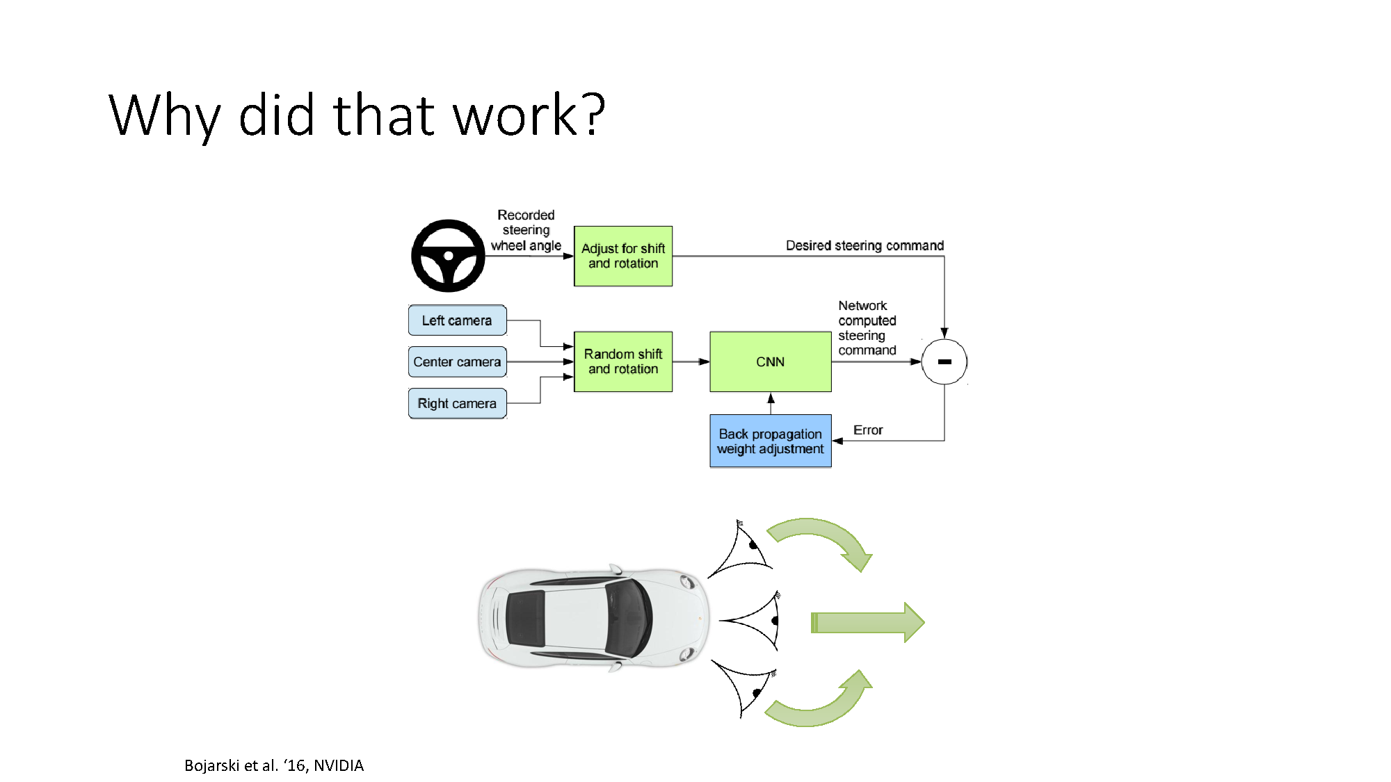
Side-camera augmentation adds states and actions that teach recovery

This also explains an apparent paradox: a dataset containing only perfect trajectories can be less useful than one containing mistakes followed by good recoveries. A closed-loop policy needs both nominal behavior and a way back.

DAgger trains on learner-induced states

The direct fix is to collect labels on states the learner actually visits. DAgger stands for Dataset Aggregation:

Train a policy on the current expert-labeled dataset.
Roll out the current policy, or a mixture of learner and expert.
Ask the expert which action should be taken at the visited states.
Add those labeled states to the dataset and retrain.
Repeat.

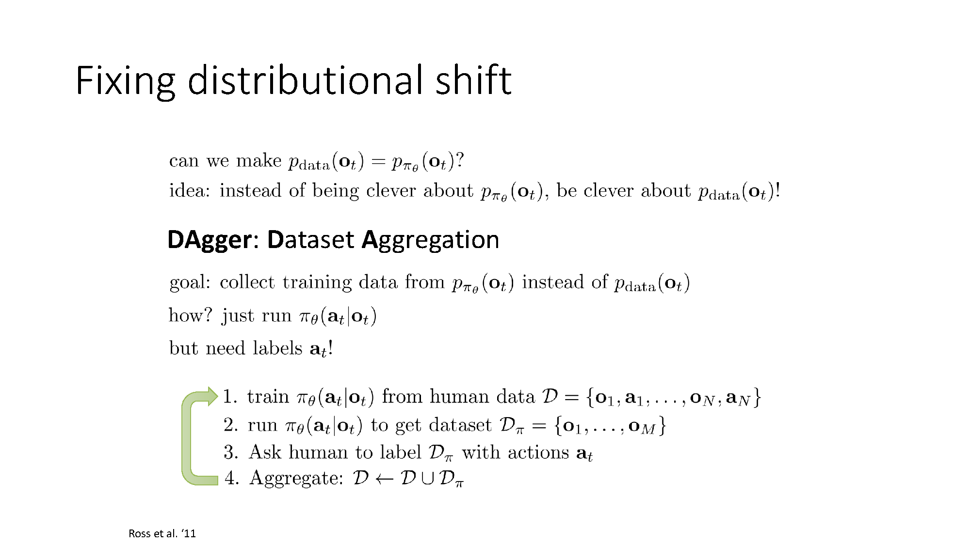
DAgger repeatedly labels states visited by the current policy and aggregates them

At iteration $k$, the new examples come from the state distribution induced by $\pi_k$, rather than only from $p_{\mathrm{train}}$. The training distribution therefore follows the learner toward the places where it needs help.

Under the assumptions used in the DAgger analysis, this changes the unfavorable horizon dependence from the BC-style worst case $O(\epsilon H^2)$ toward $O(\epsilon H)$. The important point is not the constant or the architecture. It is that the error is now trained and measured on relevant states.

DAgger does have a practical cost: the expert must label learner-generated states, and those states may be unsafe or unnatural. Mixing expert and learner actions can make early collection safer.

Intervention-only data is not identical to DAgger

A common practical variant lets the learner act until a human takes over, then stores only the intervention examples.

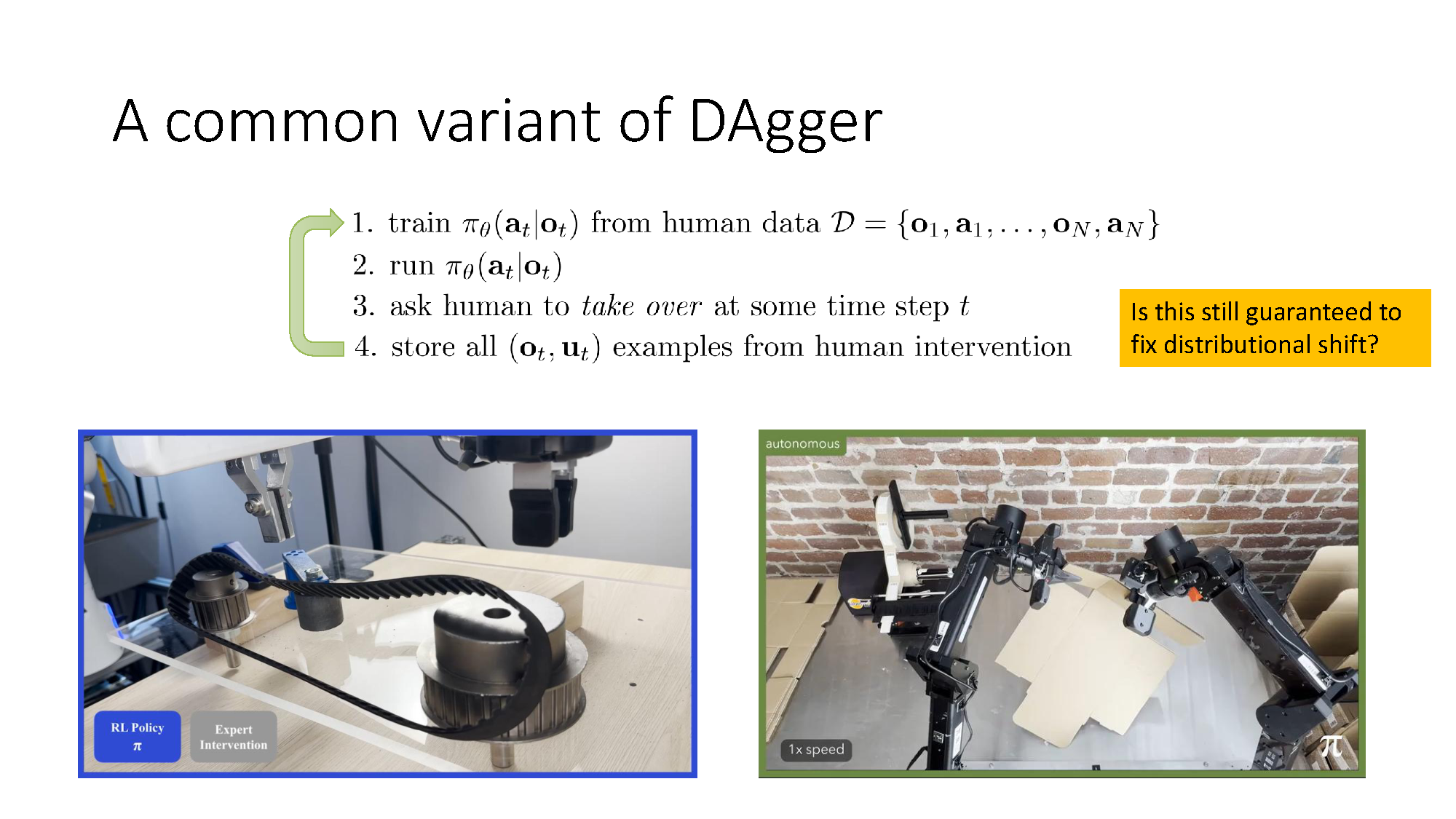
A practical DAgger-style variant stores expert takeover examples

This is useful because it concentrates labels near dangerous failures. But it does not sample all learner-visited states. Its data distribution is the intervention distribution, which depends on when the human decides to take control.

Therefore it should be understood as a practical DAgger-style method, not automatically as the same algorithm with the same guarantee. It can miss states where the policy is subtly wrong but the expert does not intervene.

What each remedy actually changes

Method	What it improves	What it does not automatically solve
Larger model or better optimizer	Lowers error on the existing dataset	Missing recovery states
More expert demonstrations	Covers more expert behavior	Learner-specific off-trajectory states
Recovery data or augmentation	Widens local state coverage	Arbitrary long-horizon shift
DAgger	Moves training data toward learner-induced states	Expert labeling cost and rollout safety

Common confusions

Does BC learn the environment dynamics?

No. BC learns an action rule from labeled examples. The dynamics still determine the data distribution encountered during rollout.

Is distributional shift just overfitting?

No. A model may generalize well on held-out expert data and still fail because deployment creates a different input distribution.

Why not simply collect more expert trajectories?

More expert data reduces error on expert states, but a nearly perfect expert rarely visits recovery states. The missing data is defined by the learner’s failures.

Does DAgger require the expert to control the system?

Not at every step. The learner can generate the states while the expert supplies counterfactual action labels. In safety-critical systems, action mixing or intervention may still be necessary.

My takeaway

Behavioral cloning is best understood as offline expert data used to train a closed-loop policy. Its objective is mathematically ordinary maximum likelihood, but its deployment distribution is created by the policy itself. That is why a tiny local error can become a large trajectory error.

The most important design question is therefore not only “How accurately can the policy copy the expert?” It is also “Does the dataset contain the states produced by the policy’s own mistakes?” Recovery data answers this locally; DAgger answers it systematically.

References

- CS285: Deep Reinforcement Learning
- Lecture 2: Supervised Learning of Behaviors (PDF)
- Stephane Ross, Geoffrey Gordon, and Drew Bagnell. A Reduction of Imitation Learning and Structured Prediction to No-Regret Online Learning, AISTATS 2011.
- Mariusz Bojarski et al. End to End Learning for Self-Driving Cars, 2016.