CS285 DRL Notes-Lecture 3 Supervised Learning of Behaviors

This is the note for Berkeley CS285 Lecture 3. The lecture asks how to make behavioral cloning work when a small prediction error can change the future data distribution.

Strong imitation learning needs three kinds of coverage: the model must represent the expert’s decisions, the data must cover situations encountered at deployment, and the task description must let experience transfer across goals.

Behavioral cloning is only the starting point

Given expert observation-action pairs, behavioral cloning fits a policy by maximum likelihood:

\arg\max_\theta \sum_{i=1}^{N}\sum_{t=1}^{H} \log\pi_\theta\!\left(a_t^{(i)}\mid o_t^{(i)}\right).

This objective is supervised, but deployment is sequential. A small action error changes the next observation, so the policy may leave the distribution represented by $\mathcal D$.

Lecture 2 addressed this with interactive data collection such as DAgger. Lecture 3 asks a complementary question: even with a reasonable dataset, can the model express the behavior, and does the dataset teach the right behavior in enough situations?

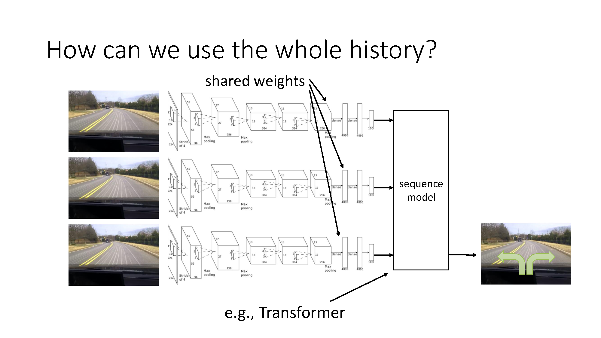
The policy may need history

A memoryless policy assumes that the current observation contains everything needed for the decision:

\pi_\theta(a_t\mid o_t).

This can fail when two identical-looking observations require different actions because of what happened earlier. The policy should then condition on history:

\pi_\theta(a_t\mid o_1,\ldots,o_t).

A sequence model shares parameters across time, so it can process a variable-length history without creating a separate model for every frame.

Using a sequence model to condition on history

More history is not automatically better. The history may contain consequences of the expert’s own actions that correlate with the next action but do not cause it. A policy can exploit these shortcuts and fail when the correlation changes. This is the causal-confusion problem.

The useful rule is: add memory when the observation is genuinely incomplete, then test whether the learned policy relies on causal information rather than convenient traces of the demonstrator.

The policy may need multiple action modes

For one observation, several expert actions can be valid. Driving around an obstacle on the left and on the right are both reasonable, but their average may drive into the obstacle.

This is why a Gaussian policy trained with mean-squared error can fail even when its prediction loss is low: it tends to represent a conditional mean rather than distinct modes.

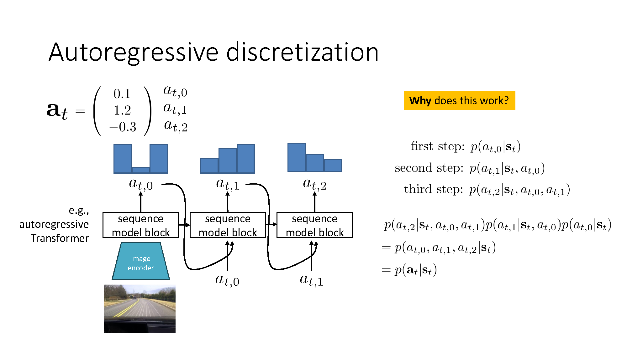
Autoregressive discretization

Discretizing an entire high-dimensional action space requires exponentially many joint bins. Instead, discretize each action dimension and predict them sequentially:

p(a_{t,2}\mid s_t,a_{t,0},a_{t,1}) p(a_{t,1}\mid s_t,a_{t,0}) p(a_{t,0}\mid s_t) =p(\mathbf a_t\mid s_t).

This is just the probability chain rule, written with the slide’s three action coordinates. The same factorization extends to any action dimension. It converts one huge joint classification problem into conditional classification problems while preserving dependence between action dimensions.

Autoregressive discretization of a continuous action

Expressive continuous policies

Another option is to keep actions continuous and use a generative distribution such as a VAE, normalizing flow, diffusion model, or flow-matching model.

The important requirement is not the model’s name. Different noise samples must actually produce different plausible action modes; otherwise the stochastic policy has collapsed back to one answer.

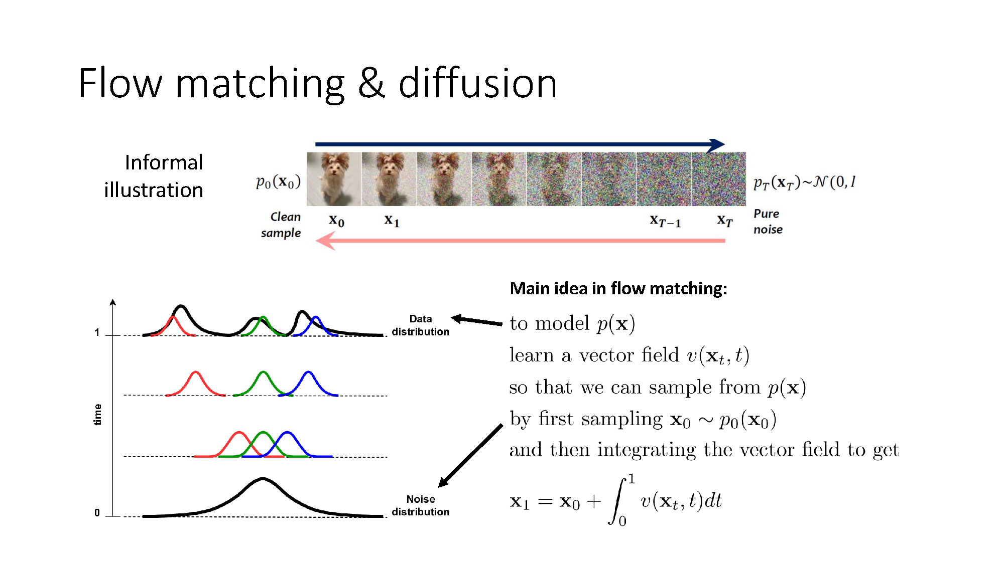
Flow matching turns noise into an action

Flow matching learns a velocity field that transports simple noise into the expert action distribution. The policy-training slide uses $\tau\in[0,1]$ for flow time here; it is not an RL trajectory.

For minibatch element $j$, sample the demonstrated pair $(o_t^{(j)},a_t^{(j)})$, noise $a_{t,0}^{(j)}\sim\mathcal N(0,I)$, and $\tau^{(j)}\sim\mathcal U(0,1)$. Interpolate exactly as in the slide:

a_{t,\tau}^{(j)} =\tau^{(j)}a_t^{(j)} +\left(1-\tau^{(j)}\right)a_{t,0}^{(j)}.

The target velocity along this straight path is $a_t^{(j)}-a_{t,0}^{(j)}$. The minibatch loss is

\mathcal L =\sum_{j=1}^{B} \left\| v_\theta\!\left(o_t^{(j)},a_{t,\tau}^{(j)},\tau^{(j)}\right) -\left(a_t^{(j)}-a_{t,0}^{(j)}\right) \right\|_2^2.

At inference, sample $a_{t,0}$ from Gaussian noise and numerically integrate the learned velocity from flow time $0$ to $1$. The endpoint is a sampled action from the learned conditional distribution.

Flow matching transports noise to the data distribution

The slide writes the parameter update with a plus sign next to the squared-error objective. For the loss written above, the correct operation is gradient descent. Equivalently, one could use gradient ascent on its negative.

Flow matching is still behavioral cloning: supervision comes from expert actions. The generative machinery changes how $\pi_\theta(a\mid o)$ is represented, not where the target behavior comes from.

Action chunking improves short-term coherence

A step-wise policy predicts one action and immediately observes again. An action-chunked policy predicts a short sequence:

a_{t:t+K}\sim \pi_\theta(a_{t:t+K}\mid o_t).

It then executes the chunk before making the next high-level prediction.

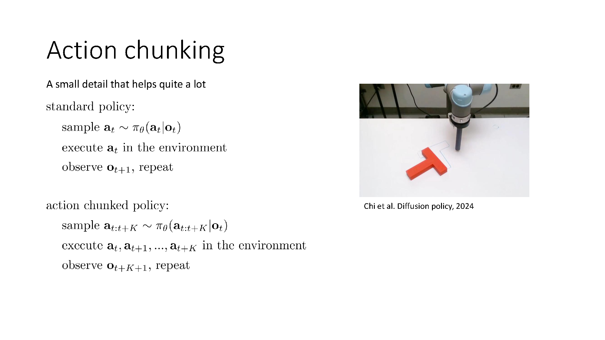
Step-wise and action-chunked policies

Chunking gives the model a direct way to represent temporally coordinated motion and reduces how often it must make a fresh decision. The tradeoff is reduced feedback inside the chunk: longer chunks are coherent but less responsive to unexpected changes.

Diffusion Policy and $\pi_0$ illustrate how expressive action distributions, chunking, and large-scale pre-training can be combined. The conceptual point is the combination, not that one specific architecture is required.

Data must teach both recovery and preference

Expert demonstrations are usually high quality but narrow: they show what to do when everything goes well, not how to recover after an error.

Two direct ways to widen coverage are:

deliberately include mistakes followed by corrections;
augment observations to show what off-trajectory situations would look like.

The correction may be more valuable than the mistake is harmful because it teaches a direction back toward the expert distribution. Still, indiscriminately cloning poor actions is not the goal.

This creates a useful distinction:

broad but suboptimal data covers many situations;
high-quality but narrow data demonstrates consistent preferred behavior.

Broad data and narrow expert data

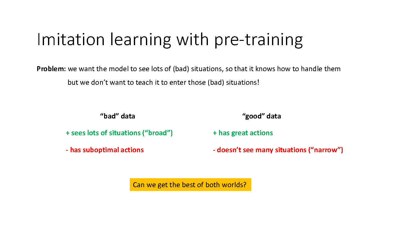
Pre-training can learn broad representations and situation awareness from diverse data. Post-training then emphasizes the high-quality actions required by the target task. Broad data supplies coverage; narrow data supplies preference.

This is a tendency, not a guarantee. If pre-training teaches strong harmful correlations or post-training is too weak, more data can still make the final policy worse.

Goals turn many tasks into one conditional problem

A separate policy for every destination wastes shared experience. A goal-conditioned policy uses one model:

\pi_\theta(a\mid s,g).

For demonstration $i$ ending at $s_T^{i}$, the slide relabels its goal as $g=s_T^{i}$ and trains

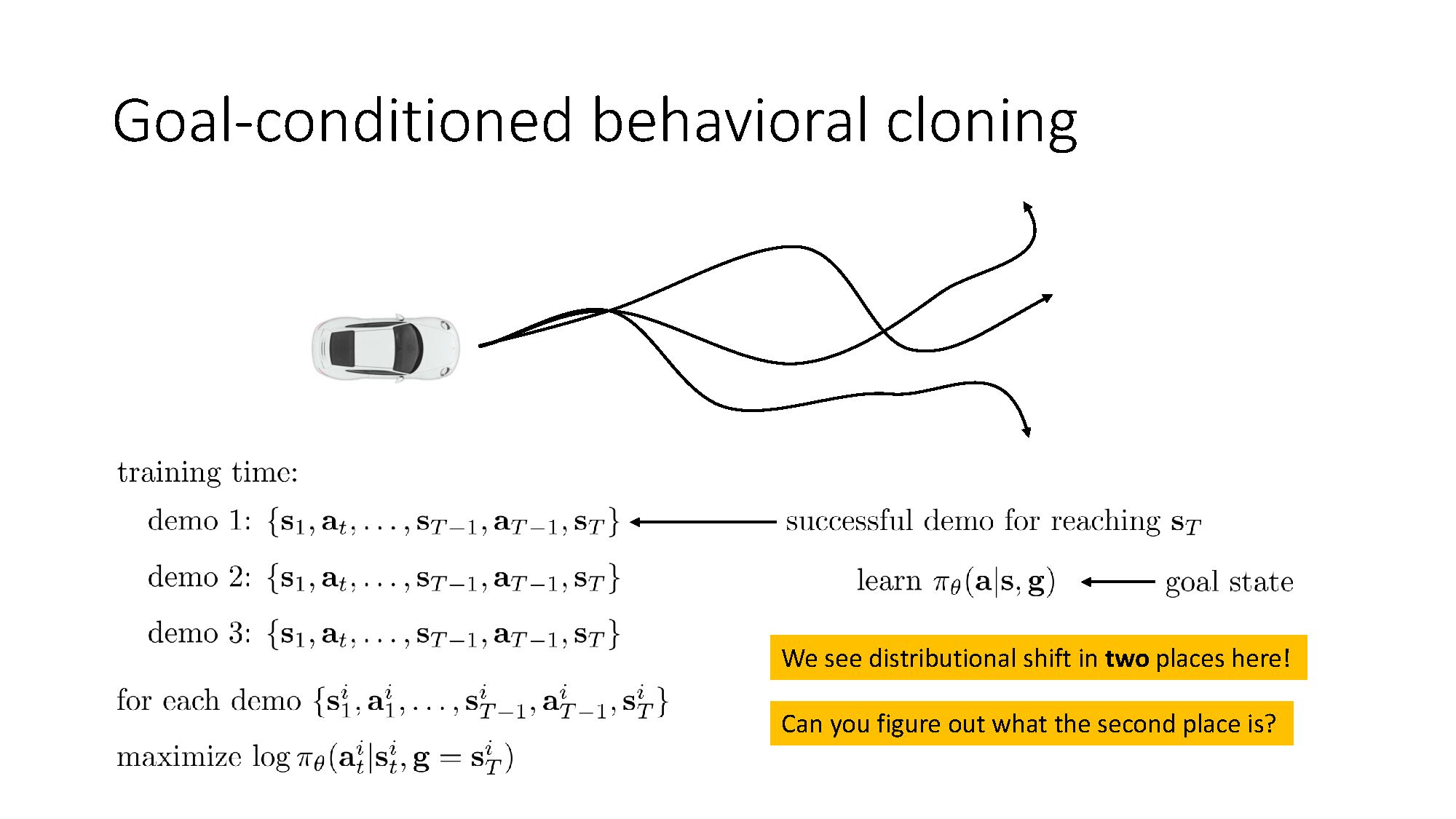
\text{maximize}\quad \log\pi_\theta\!\left(a_t^{i}\mid s_t^{i},g=s_T^{i}\right).

Goal-conditioned behavioral cloning

Goal conditioning enables parameter sharing, but it does not automatically solve distribution shift. There are now two shifts to consider:

the policy may visit states that demonstrations did not cover;
test-time state-goal pairs may differ from the pairs seen together during training.

Learning many tasks becomes easier only when their data share useful structure and cover the combinations needed at deployment.

Relabel what a trajectory actually achieved

A rollout that misses its intended goal is not necessarily useless. It is still a demonstration of how to reach the states that it actually visited.

This gives a supervised improvement loop:

collect rollouts with the current policy;
relabel achieved states as goals;
train the goal-conditioned policy on the relabeled data;
collect new rollouts and repeat.

Iterated goal relabeling

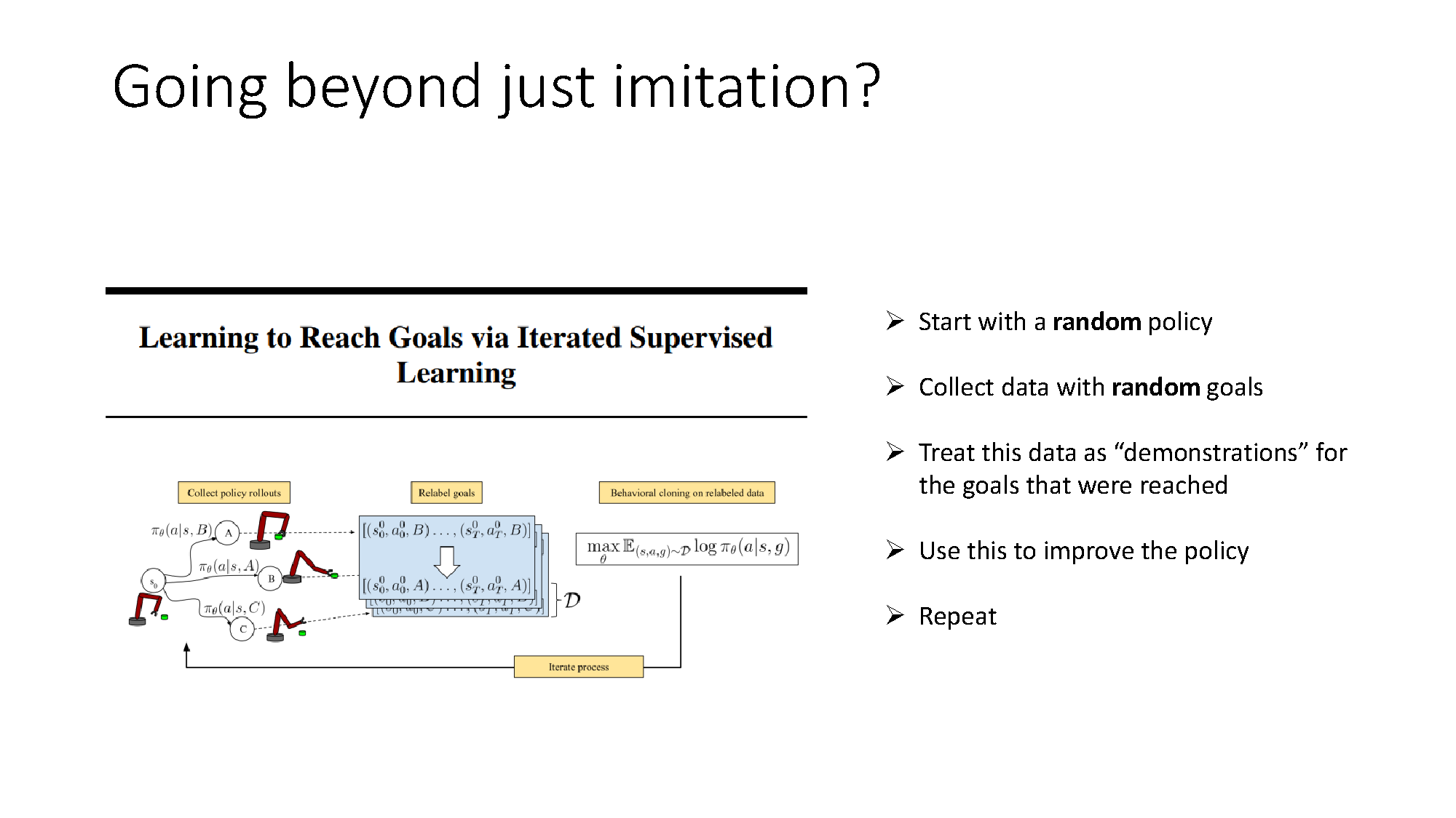
The key insight is hindsight: judge a trajectory against what it achieved, not only against what was originally requested. This idea later reappears in reinforcement learning as hindsight experience replay.

Relabeling improves data reuse, but it cannot invent experience for goals the policy never reaches. Exploration and coverage remain necessary.

Common confusions

History is not always useful context. It helps partial observability but can also expose spurious correlations.
Multimodal does not mean noisy. Multiple actions can each be coherent solutions; their average may be invalid.
Flow matching is not reinforcement learning. Here it is a supervised way to represent a behavioral-cloning policy.
Broad data is not automatically good policy data. It provides coverage; high-quality post-training determines preferred behavior.
Goal conditioning is not planning by itself. It maps a current state and goal to actions, using patterns learned from data.

My takeaway

Lecture 3 is a study of coverage. Sequence models cover missing temporal context. Autoregressive and generative policies cover multiple valid actions. Recovery data and pre-training cover more situations. Goal conditioning covers more tasks with shared parameters.

None of these removes the sequential nature of imitation learning. The learned policy still creates its own future inputs. Better models reduce approximation error, and better data reduce surprise, but deployment succeeds only when representation and coverage work together.